Predicting Climbing Accident Outcomes from Article Sentiment

I used NLP techniques and different ML models to predict the outcome of climbing accidents.

Author

Affiliation

Andrew Bartnik

Master of Environmental Data Science Program @ The Bren School (UCSB)

Preprocessing

Here, we are going to predict the outcome of climbing incidents (fatal or nonfatal) using text from climbing incident articles. This data set includes more possible predictors than the text alone, but for this model we will only use the text variable.

urlfile ="https://raw.githubusercontent.com/MaRo406/EDS-231-text-sentiment/main/data/climbing_reports_model_dat.csv"
incidents_df<-readr::read_csv(url(urlfile))
head(incidents_df)

# A tibble: 6 × 5
  ID    `Accident Title`                                    Publi…¹ Text  Deadly
  <chr> <chr>                                                 <dbl> <chr>  <dbl>
1 1     Failure of Rappel Setup (Protection Pulled Out), I…    1990 "Col…     NA
2 2     Failure of Rappel—Failure to Check System, British…    1990 "Bri…     NA
3 3     Fall into Crevasse, Climbing Alone, Inadequate Equ…    1990 "Alb…     NA
4 4     Fall into Crevasse, Climbing Unroped, British Colu…    1990 "Bri…     NA
5 5     Fall Into Crevasse, Unroped, Inadequate Equipment,…    1990 "On …      1
6 6     Fall into Moat, Descending Unroped, Poor Position,…    1990 "Alb…      1
# … with abbreviated variable name ¹​`Publication Year`

We’ll split our data into training and test portions

set.seed(1234)

# Adding a fatality binary indicator
incidents2class <- incidents_df |> 
  mutate(fatal = factor(if_else(
    is.na(Deadly) ,
    "non-fatal", "fatal")))

# Splitting our data, stratifying on the outcome
incidents_split <- initial_split(incidents2class, strata = fatal)

# Now for making our training and testing sets:
incidents_train <- training(incidents_split)
incidents_test <- testing(incidents_split)

We use recipe() from tidymodels to specify the predictor and outcome variables and the data.

# Making the recipe. We're saying we want to predict fatal by using Text
incidents_rec <- recipe(fatal ~ Text, data = incidents_train)

Next we add some familiar pre-processing steps on our Text variable. We first tokenize the articles to word level, filter to the most common words, and calculate tf-idf.

# Adding steps to our recipe
recipe <- incidents_rec %>%
  step_tokenize(Text) %>% 
  step_tokenfilter(Text, max_tokens = 1000) %>%
  step_tfidf(Text) #new one from textrecipes

Modeling

We use tidymodels workflow to combine the modeling components. There are several advantages of doing this: We don’t have to keep track of separate objects in our workspace. The recipe prepping and model fitting can be executed using a single call to fit() . If we have custom tuning parameter settings, these can be defined using a simpler interface when combined with tune.

Naive Bayes

# Making the workflow object
incidents_wf <- workflow() %>%
  add_recipe(recipe)

We want to use Naive Bayes to classify the outcomes.

nb_spec <- naive_Bayes() %>%
  set_mode("classification") %>% #set modeling context
  set_engine("naivebayes") #method for fitting model

nb_spec

Naive Bayes Model Specification (classification)

Computational engine: naivebayes 

Now we are ready to add our model to the workflow and fit it to the training data

# Fitting the model to our workflow
nb_fit <- incidents_wf %>%
  add_model(nb_spec) %>%
  fit(data = incidents_train)

Next up is model evaluation. We’ll stretch our training data further and use resampling to evaluate our Naive Bayes model. Here we create 10-fold cross-validation sets, and use them to estimate performance.

# Set the seed for reproducibility
set.seed(234)
incidents_folds <- vfold_cv(incidents_train) #default is v = 10

incidents_folds

#  10-fold cross-validation 
# A tibble: 10 × 2
   splits             id    
   <list>             <chr> 
 1 <split [1869/208]> Fold01
 2 <split [1869/208]> Fold02
 3 <split [1869/208]> Fold03
 4 <split [1869/208]> Fold04
 5 <split [1869/208]> Fold05
 6 <split [1869/208]> Fold06
 7 <split [1869/208]> Fold07
 8 <split [1870/207]> Fold08
 9 <split [1870/207]> Fold09
10 <split [1870/207]> Fold10

nb_wf <- workflow() %>%
  add_recipe(recipe) %>%
  add_model(nb_spec)

nb_wf

══ Workflow ════════════════════════════════════════════════════════════════════
Preprocessor: Recipe
Model: naive_Bayes()

── Preprocessor ────────────────────────────────────────────────────────────────
3 Recipe Steps

• step_tokenize()
• step_tokenfilter()
• step_tfidf()

── Model ───────────────────────────────────────────────────────────────────────
Naive Bayes Model Specification (classification)

Computational engine: naivebayes 

To estimate its performance, we fit the model many times, once to each of these resampled folds, and then evaluate on the holdout part of each resampled fold.

nb_rs <- fit_resamples(
  nb_wf,
  incidents_folds,
  control = control_resamples(save_pred = TRUE)
)

We then extract the relevant information using collect_metrics() and collect_predictions() and examine the performance metrics.

nb_rs_metrics <- collect_metrics(nb_rs)
nb_rs_predictions <- collect_predictions(nb_rs)
nb_rs_metrics

# A tibble: 2 × 6
  .metric  .estimator  mean     n std_err .config             
  <chr>    <chr>      <dbl> <int>   <dbl> <chr>               
1 accuracy binary     0.800    10 0.00474 Preprocessor1_Model1
2 roc_auc  binary     0.730    10 0.0118  Preprocessor1_Model1

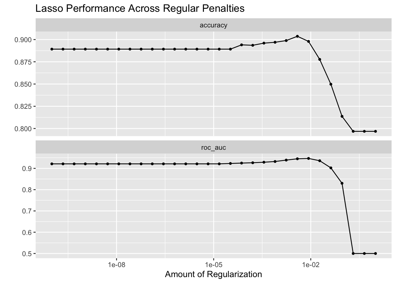
We’ll use two performance metrics: accuracy and ROC AUC. Accuracy is the proportion of the data that is predicted correctly. The ROC curve plots the true positive rate against the false positive rate; AUC closer to 1 indicates a better-performing model, while AUC closer to 0.5 indicates a model that does no better than random guessing.

nb_rs_predictions %>%
  group_by(id) %>%
  roc_curve(truth = fatal, .pred_fatal) %>%
  autoplot() +
  labs(
    "Resamples",
    title = "ROC curve for Climbing Incident Reports"
  )

Another model method involves the confusion matrix. A confusion matrix tabulates a model’s false positives and false negatives for each class.

conf_mat_resampled(nb_rs, tidy = FALSE) %>% #compute matrix for each fold then average
  autoplot(type = "heatmap")

Lasso Regression

Now, lets try a different model - lasso regression to see if we can score better. We follow the same approach that we did for the Naive Bayes model.

# Specifying the model
lasso_spec <- logistic_reg(penalty = 0.01, mixture =1) |> 
  set_mode('classification') |> 
  set_engine("glmnet")

# Making the workflow  
lasso_wf <- workflow() |> 
  add_recipe(recipe) |> 
  add_model(lasso_spec)

lasso_wf

══ Workflow ════════════════════════════════════════════════════════════════════
Preprocessor: Recipe
Model: logistic_reg()

── Preprocessor ────────────────────────────────────────────────────────────────
3 Recipe Steps

• step_tokenize()
• step_tokenfilter()
• step_tfidf()

── Model ───────────────────────────────────────────────────────────────────────
Logistic Regression Model Specification (classification)

Main Arguments:
  penalty = 0.01
  mixture = 1

Computational engine: glmnet 

We then fit the model to the resamples, and collect our metrics

set.seed(123)
lasso_rs <- fit_resamples(
  lasso_wf,
  incidents_folds,
  control = control_resamples(save_pred = T)
)

lasso_rs_metrics <- collect_metrics(lasso_rs)
lasso_rs_predictions <- collect_predictions(lasso_rs)
lasso_rs_metrics

# A tibble: 2 × 6
  .metric  .estimator  mean     n std_err .config             
  <chr>    <chr>      <dbl> <int>   <dbl> <chr>               
1 accuracy binary     0.895    10 0.00538 Preprocessor1_Model1
2 roc_auc  binary     0.947    10 0.00593 Preprocessor1_Model1

Now we can check our predictions:

lasso_rs_predictions |> 
  group_by(id) |> 
  roc_curve(truth = fatal, .pred_fatal) |> 
  autoplot() + labs(color = "Resamples",
                    title = "ROC for Climbing Incident Reports")

Logistic Regression

Now for Logistic Regression:

log_spec <- logistic_reg(penalty = tune(), mixture = 1) |> set_mode("classification") |> set_engine("glmnet")
log_wf <- workflow() |> 
  add_recipe(recipe) |> 
  add_model(log_spec)

set.seed(123)
lambda_grid <- grid_regular(penalty(), levels = 30)
log_rs <- tune_grid(log_wf, incidents_folds, grid = lambda_grid, control = control_resamples(save_pred = T))

Lets evaluate our Logistic Regression model:

# Collecting metrics
collect_metrics(log_rs)

# A tibble: 60 × 7
    penalty .metric  .estimator  mean     n std_err .config              
      <dbl> <chr>    <chr>      <dbl> <int>   <dbl> <chr>                
 1 1   e-10 accuracy binary     0.889    10 0.00644 Preprocessor1_Model01
 2 1   e-10 roc_auc  binary     0.921    10 0.00613 Preprocessor1_Model01
 3 2.21e-10 accuracy binary     0.889    10 0.00644 Preprocessor1_Model02
 4 2.21e-10 roc_auc  binary     0.921    10 0.00613 Preprocessor1_Model02
 5 4.89e-10 accuracy binary     0.889    10 0.00644 Preprocessor1_Model03
 6 4.89e-10 roc_auc  binary     0.921    10 0.00613 Preprocessor1_Model03
 7 1.08e- 9 accuracy binary     0.889    10 0.00644 Preprocessor1_Model04
 8 1.08e- 9 roc_auc  binary     0.921    10 0.00613 Preprocessor1_Model04
 9 2.40e- 9 accuracy binary     0.889    10 0.00644 Preprocessor1_Model05
10 2.40e- 9 roc_auc  binary     0.921    10 0.00613 Preprocessor1_Model05
# … with 50 more rows

autoplot(log_rs) + labs(title = "Lasso Performance Across Regular Penalties")

log_rs |> show_best("roc_auc")

# A tibble: 5 × 7
   penalty .metric .estimator  mean     n std_err .config              
     <dbl> <chr>   <chr>      <dbl> <int>   <dbl> <chr>                
1 0.00853  roc_auc binary     0.947    10 0.00586 Preprocessor1_Model24
2 0.00386  roc_auc binary     0.945    10 0.00532 Preprocessor1_Model23
3 0.00174  roc_auc binary     0.939    10 0.00500 Preprocessor1_Model22
4 0.0189   roc_auc binary     0.936    10 0.00596 Preprocessor1_Model25
5 0.000788 roc_auc binary     0.932    10 0.00527 Preprocessor1_Model21

log_rs |> show_best("accuracy")

# A tibble: 5 × 7
   penalty .metric  .estimator  mean     n std_err .config              
     <dbl> <chr>    <chr>      <dbl> <int>   <dbl> <chr>                
1 0.00386  accuracy binary     0.904    10 0.00581 Preprocessor1_Model23
2 0.00174  accuracy binary     0.899    10 0.00672 Preprocessor1_Model22
3 0.00853  accuracy binary     0.898    10 0.00516 Preprocessor1_Model24
4 0.000788 accuracy binary     0.897    10 0.00624 Preprocessor1_Model21
5 0.000356 accuracy binary     0.896    10 0.00648 Preprocessor1_Model20

Using our best model, we perform a final fit and evaluate its performance:

# Finalizing the workflow. extracting the metrics
chosen_acc <- log_rs |> select_by_one_std_err(metric= "accuracy", -penalty)
final_log <- finalize_workflow(log_wf, chosen_acc)
final_log <- fit(final_log, incidents_train)
final_log |> extract_fit_parsnip() |> tidy() |> arrange(estimate)

# A tibble: 1,001 × 3
   term                 estimate penalty
   <chr>                   <dbl>   <dbl>
 1 tfidf_Text_died        -277.  0.00853
 2 tfidf_Text_body        -158.  0.00853
 3 tfidf_Text_death       -132.  0.00853
 4 tfidf_Text_fatal        -76.8 0.00853
 5 tfidf_Text_breathing    -47.7 0.00853
 6 tfidf_Text_past         -32.5 0.00853
 7 tfidf_Text_observed     -32.5 0.00853
 8 tfidf_Text_occurred     -31.7 0.00853
 9 tfidf_Text_noticed      -31.1 0.00853
10 tfidf_Text_either       -31.0 0.00853
# … with 991 more rows

last_fit(final_log, incidents_split) |> collect_metrics()

# A tibble: 2 × 4
  .metric  .estimator .estimate .config             
  <chr>    <chr>          <dbl> <chr>               
1 accuracy binary         0.916 Preprocessor1_Model1
2 roc_auc  binary         0.951 Preprocessor1_Model1

Random Forest Classifier

Now we’re going to try a more powerful algorithm: the random forest classifier.

# Specifying the model
rf_spec <- rand_forest() |> set_mode("classification") |> set_engine("ranger")

We’re first going to conduct an initial out-of-the-box model fit on the training data and prediction on the test test data. Assess the performance of this initial model.

# Initializing a workflow, fitting it to resamples
rf_workflow <- workflow() |> add_recipe(recipe) |> add_model(rf_spec)
rf_fit <- rf_workflow |> fit(data = incidents_train)

rf_rs <- fit_resamples(
  rf_workflow,
  incidents_folds,
  control = control_resamples(save_pred = TRUE)
)

rf_rs_metrics <- collect_metrics(rf_rs)
nb_rs_predictions <- collect_predictions(rf_rs)
rf_rs_metrics

# A tibble: 2 × 6
  .metric  .estimator  mean     n std_err .config             
  <chr>    <chr>      <dbl> <int>   <dbl> <chr>               
1 accuracy binary     0.867    10 0.00668 Preprocessor1_Model1
2 roc_auc  binary     0.947    10 0.00400 Preprocessor1_Model1

Initial model has an accuracy of 86% and roc_auc of 0.95. Not bad at all.

Now, we’re going to tune the hyperparameters:

# specifying which parameters to tune, adding this new model back into a workflow
tune_rf_spec <- rand_forest(trees = tune(), mtry = tune(), min_n = tune()) |> set_mode("classification") |> set_engine("ranger")
tune_rf_wf <- workflow() |> 
  add_recipe(recipe) |> 
  add_model(tune_rf_spec)

set.seed(123)
randf_grid <-grid_regular(trees(), min_n(), mtry(range(1:13)))
doParallel::registerDoParallel() # running this in parallel

tune_rs <- tune_grid(tune_rf_wf, incidents_folds, grid = randf_grid, control = control_resamples(save_pred = T, parallel_over = 'everything'))

We then conduct a model fit using your newly tuned model specification and investigate the terms most highly associated with non-fatal, and fatal reports

# extracting our best hyperparameters:
params <- tune_rs |> show_best("accuracy") |> slice(1) |> select(trees, mtry, min_n)
best_trees_rf <- params$trees
best_mtry_rf <- params$mtry
best_min_n_rf <- params$min_n

# Final model using our best parameters
randf_final <- rand_forest(
  trees = best_trees_rf,
  mtry = best_mtry_rf,
  min_n = best_min_n_rf
) |>
  set_mode("classification") |>
  set_engine("ranger")


# fit on the training
randf_final_fit <- tune_rf_wf |> 
  update_model(randf_final) |> 
  fit(data = incidents_train)

Unfortunately tidy doesnt support ranger and we are unable to see variable importance/terms most highly associated with different reports

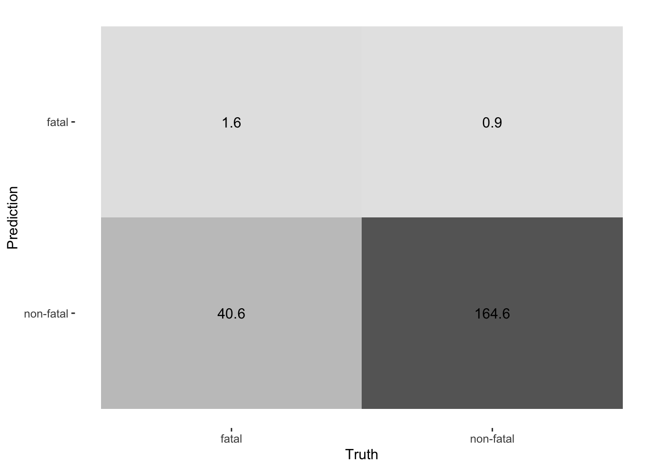
Now, we’ll predict fatality of the reports in the test set. We can compare this prediction performance to that of the Naive Bayes and Lasso models.

# predict on the test, calculate RMSE
rf_testing_preds <- predict(randf_final_fit, incidents_test) |> 
  bind_cols(incidents_test) |> 
  mutate(truth = as.factor(fatal), estimate = as.factor(.pred_class)) |> 
  metrics(truth = truth, estimate = estimate)

rf_testing_preds

# A tibble: 2 × 3
  .metric  .estimator .estimate
  <chr>    <chr>          <dbl>
1 accuracy binary         0.812
2 kap      binary         0.119

Unfortunately, our predictions got worse as we tuned the model. This could be due to bad combinations chosen by the grid space, which is likely since our tuning grid isn’t very big. Our random forest model also performs worse than the lasso model (which scored 92% accuracy), but slightly better than the Naive Bayes model (81% accuracy)

Embeddings

First, let’s calculate the unigram probabilities – how often we see each word in this corpus.

unigram_probs <- incidents_df |> unnest_tokens(word, Text) |> anti_join(stop_words, by = 'word') |> count(word, sort=T) |> mutate(p = n/sum(n))
unigram_probs

# A tibble: 25,205 × 3
   word         n       p
   <chr>    <int>   <dbl>
 1 rope      5129 0.00922
 2 feet      5101 0.00917
 3 climbing  4755 0.00855
 4 route     4357 0.00783
 5 climbers  3611 0.00649
 6 climb     3209 0.00577
 7 fall      3168 0.00569
 8 climber   2964 0.00533
 9 rescue    2928 0.00526
10 source    2867 0.00515
# … with 25,195 more rows

So now we have the probability of each word.

Next, we need to know how often we find each word near each other word – the skipgram probabilities. In this case we’ll define the word context as a five-word window. We’ll slide that window across all of our text and record which words occur together within that window. Let’s write some code that adds an ngramID column that contains constituent information about each 5-gram we constructed by sliding our window.

skipgrams <- incidents_df |> unnest_tokens(ngram, Text, token = "ngrams", n = 5) |> mutate(ngramID = row_number()) |> tidyr::unite(skipgramID, ID, ngramID) |> unnest_tokens(word, ngram) |> anti_join(stop_words, by = 'word')

Now we use widyr::pairwise_count() to sum the total # of occurrences of each pair of words.

#calculate probabilities
skipgram_probs <- skipgrams |> pairwise_count(word, skipgramID,diag = T, sort = T) |> mutate(p = n/sum(n))

The next step is to normalize these probabilities, that is, to calculate how often words occur together within a window, relative to their total occurrences in the data.

normalized_prob <- skipgram_probs |> filter(n>20) |> rename(word1 = item1, word2=item2) |> left_join(unigram_probs |> select(word1 = word, p1 = p), by = 'word1') |> 
  left_join(unigram_probs |> select(word2 = word, p2 = p), by = 'word2') |> mutate(p_together = p/p1/p2)

normalized_prob

# A tibble: 31,240 × 7
   word1    word2        n       p      p1      p2 p_together
   <chr>    <chr>    <dbl>   <dbl>   <dbl>   <dbl>      <dbl>
 1 rope     rope     25494 0.00340 0.00922 0.00922       40.0
 2 feet     feet     25331 0.00338 0.00917 0.00917       40.2
 3 climbing climbing 23320 0.00311 0.00855 0.00855       42.6
 4 route    route    21696 0.00289 0.00783 0.00783       47.2
 5 climbers climbers 17912 0.00239 0.00649 0.00649       56.7
 6 climb    climb    15998 0.00213 0.00577 0.00577       64.2
 7 fall     fall     15705 0.00210 0.00569 0.00569       64.6
 8 climber  climber  14660 0.00196 0.00533 0.00533       68.9
 9 rescue   rescue   14003 0.00187 0.00526 0.00526       67.5
10 rock     rock     13846 0.00185 0.00506 0.00506       72.3
# … with 31,230 more rows

Now we have all the pieces to calculate the point-wise mutual information (PMI) measure. It’s the logarithm of the normalized probability of finding two words together. PMI tells us which words occur together more often than expected based on how often they occurred on their own.

Then we convert to a matrix so we can use matrix factorization and reduce the dimensionality of the data.

pmi_matrix <- normalized_prob |> mutate(pmi = log10(p_together)) |> cast_sparse(word1, word2, pmi)

We do the singluar value decomposition with irlba::irlba(). It’s a “partial decomposition” as we are specifying a limited number of dimensions, in this case 100.

pmi_matrix@x[is.na(pmi_matrix@x)]<0

logical(0)

pmi_svd <- irlba(pmi_matrix, 100, maxit = 500)
word_vectors <- pmi_svd$u

rownames(word_vectors) <- rownames(pmi_matrix)

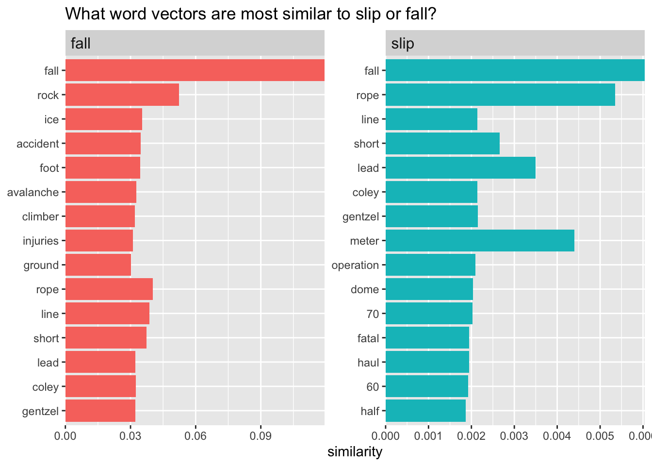
These vectors in the “u” matrix are contain “left singular values”. They are orthogonal vectors that create a 100-dimensional semantic space where we can locate each word. The distance between words in this space gives an estimate of their semantic similarity.

Here’s a function written by Julia Silge for matching the most similar vectors to a given vector.

search_synonyms <- function(word_vectors, selected_vector) {
dat <- word_vectors %*% selected_vector
    
similarities <- dat %>%
        tibble(token = rownames(dat), similarity = dat[,1])

similarities %>%
       arrange(-similarity) %>%
        select(c(2,3))
}

Let’s test it out!

fall <- search_synonyms(word_vectors = word_vectors, word_vectors['fall',])
fall

# A tibble: 9,104 × 2
   token     similarity
   <chr>          <dbl>
 1 fall          0.119 
 2 rock          0.0524
 3 rope          0.0403
 4 line          0.0387
 5 short         0.0374
 6 ice           0.0354
 7 accident      0.0347
 8 foot          0.0345
 9 avalanche     0.0326
10 coley         0.0324
# … with 9,094 more rows

slip <- search_synonyms(word_vectors = word_vectors, word_vectors['slip',])
slip

# A tibble: 9,104 × 2
   token     similarity
   <chr>          <dbl>
 1 fall         0.00604
 2 rope         0.00535
 3 meter        0.00440
 4 lead         0.00349
 5 short        0.00266
 6 gentzel      0.00215
 7 coley        0.00214
 8 line         0.00214
 9 operation    0.00209
10 dome         0.00203
# … with 9,094 more rows

ice <- search_synonyms(word_vectors = word_vectors, word_vectors['ice',])
ice

# A tibble: 9,104 × 2
   token    similarity
   <chr>         <dbl>
 1 ice          0.307 
 2 crampons     0.143 
 3 axe          0.0932
 4 axes         0.0905
 5 ax           0.0882
 6 snow         0.0831
 7 boots        0.0753
 8 tools        0.0711
 9 wearing      0.0710
10 screws       0.0680
# … with 9,094 more rows

Here’s a plot for visualizing the most similar words to a given target word.

slip %>%
    mutate(selected = "slip") %>%
    bind_rows(fall %>%
                  mutate(selected = "fall")) %>%
    group_by(selected) %>%
    top_n(15, similarity) %>%
    ungroup %>%
    mutate(token = reorder(token, similarity)) %>%
    ggplot(aes(token, similarity, fill = selected)) +
    geom_col(show.legend = FALSE) +
    facet_wrap(~selected, scales = "free") +
    coord_flip() +
    theme(strip.text=element_text(hjust=0, size=12)) +
    scale_y_continuous(expand = c(0,0)) +
    labs(x = NULL, title = "What word vectors are most similar to slip or fall?")

One of the cool things about representing words as numerical vectors is that we can use math on those numbers that has some semantic meaning.

snow_danger <- word_vectors["snow",] + word_vectors["danger",]
search_synonyms(word_vectors, snow_danger)

# A tibble: 9,104 × 2
   token      similarity
   <chr>           <dbl>
 1 snow           0.396 
 2 avalanche      0.131 
 3 conditions     0.0918
 4 soft           0.0806
 5 wet            0.0783
 6 ice            0.0769
 7 icy            0.0735
 8 slope          0.0703
 9 fresh          0.0604
10 blindness      0.0596
# … with 9,094 more rows

no_snow_danger <- word_vectors["danger",] - word_vectors["snow",]
search_synonyms(word_vectors, no_snow_danger)

# A tibble: 9,104 × 2
   token     similarity
   <chr>          <dbl>
 1 avalanche     0.0882
 2 danger        0.0547
 3 rockfall      0.0540
 4 gulch         0.0534
 5 class         0.0507
 6 hazard        0.0403
 7 hazards       0.0394
 8 occurred      0.0376
 9 potential     0.0373
10 mph           0.0361
# … with 9,094 more rows

Embeddings in Biodiversity Lexus

Now we’ll use the data from our Nexis Uni query from Week 2, to create a set of word embeddings. We’ll take essentially the same steps we did previously

pre_files <- list.files(pattern = ".docx", 
                        path = "~/Desktop/misc/MEDS/Spring/text/text_analysis/data/lab2/files2",
                       full.names = TRUE, 
                       recursive = TRUE, 
                       ignore.case = TRUE)


pre_dat <- lnt_read(pre_files)

Creating LNToutput from 101 files...

    ...files loaded [0.26 secs]

    ...articles split [0.28 secs]

    ...lengths extracted [0.29 secs]

    ...headlines extracted [0.29 secs]

    ...newspapers extracted [0.29 secs]

    ...dates extracted [0.30 secs]

    ...authors extracted [0.31 secs]

    ...sections extracted [0.31 secs]

    ...editions extracted [0.31 secs]

Warning in lnt_asDate(date.v, ...): More than one language was detected. The
most likely one was chosen (English 99%)

    ...dates converted [0.32 secs]

    ...metadata extracted [0.32 secs]

    ...article texts extracted [0.32 secs]

    ...superfluous whitespace removed [0.33 secs]

Elapsed time: 0.33 secs

meta <- pre_dat@meta
articles <- pre_dat@articles
paragraphs <- pre_dat@paragraphs

data <- tibble(Date = meta$Date, Headline = meta$Headline, id = pre_dat@articles$ID, text = pre_dat@articles$Article)

unigram_probs_lexis <- data |> unnest_tokens(word, text) |> anti_join(stop_words, by = 'word') |> count(word, sort=T) |> mutate(p = n/sum(n))
unigram_probs_lexis

# A tibble: 6,528 × 3
   word              n       p
   <chr>         <int>   <dbl>
 1 biodiversity    866 0.0292 
 2 species         238 0.00801
 3 climate         173 0.00582
 4 conservation    162 0.00545
 5 diversity       146 0.00491
 6 nature          145 0.00488
 7 environment     141 0.00475
 8 water           137 0.00461
 9 environmental   128 0.00431
10 natural         128 0.00431
# … with 6,518 more rows

lexis_skipgrams <- data |> unnest_tokens(ngram, text, token = "ngrams", n = 5) |> mutate(ngramID = row_number()) |> tidyr::unite(skipgramID, id, ngramID) |> unnest_tokens(word, ngram) |> anti_join(stop_words, by = 'word')

#calculate probabilities
lexis_skipgram_probs <- lexis_skipgrams |> pairwise_count(word, skipgramID,diag = T, sort = T) |> mutate(p = n/sum(n))

norm_prob_lexis <- lexis_skipgram_probs |> 
  filter(n>20) |> 
  rename(word1 = item1, word2=item2) |> 
  left_join(unigram_probs_lexis |> select(word1 = word, p1 = p), by = 'word1') |> 
  left_join(unigram_probs_lexis |> select(word2 = word, p2 = p), by = 'word2') |> mutate(p_together = p/p1/p2)

pmi_matrix_lexis <- norm_prob_lexis |> mutate(pmi = log10(p_together)) |> cast_sparse(word1, word2, pmi)
pmi_matrix_lexis@x[is.na(pmi_matrix_lexis@x)]<0

logical(0)

pmi_svd <- irlba(pmi_matrix_lexis, 100, maxit = 500)
word_vectors_lexis <- pmi_svd$u

rownames(word_vectors_lexis) <- rownames(pmi_matrix_lexis)

We can take 3-5 key words in our data set to calculate and plot the 10 most semantically similar words for each of them.

biodiversity, climate, species, nature, and change

biodiversity <- search_synonyms(word_vectors = word_vectors_lexis, word_vectors_lexis['biodiversity',])
biodiversity

# A tibble: 1,395 × 2
   token        similarity
   <chr>             <dbl>
 1 biodiversity     0.357 
 2 hotspots         0.152 
 3 threats          0.127 
 4 council          0.111 
 5 view             0.102 
 6 conserve         0.0981
 7 assessment       0.0943
 8 funds            0.0926
 9 framework        0.0926
10 board            0.0919
# … with 1,385 more rows

climate <- search_synonyms(word_vectors = word_vectors_lexis, word_vectors_lexis['climate',])
climate

# A tibble: 1,395 × 2
   token        similarity
   <chr>             <dbl>
 1 climate         0.396  
 2 nexus           0.374  
 3 crisis          0.229  
 4 change          0.206  
 5 environment     0.0614 
 6 minister        0.0169 
 7 protecting      0.0125 
 8 biodiversity    0.00732
 9 local           0.00278
10 fund            0.00187
# … with 1,385 more rows

species <- search_synonyms(word_vectors = word_vectors_lexis, word_vectors_lexis["species",])
species

# A tibble: 1,395 × 2
   token      similarity
   <chr>           <dbl>
 1 species        0.382 
 2 keystone       0.238 
 3 invasive       0.227 
 4 richness       0.198 
 5 animal         0.127 
 6 endangered     0.125 
 7 threatened     0.125 
 8 plant          0.123 
 9 extinction     0.0867
10 wild           0.0795
# … with 1,385 more rows

nature <- search_synonyms(word_vectors = word_vectors_lexis, word_vectors_lexis['nature',])
nature

# A tibble: 1,395 × 2
   token         similarity
   <chr>              <dbl>
 1 nature            0.297 
 2 positive          0.248 
 3 related           0.235 
 4 based             0.150 
 5 issues            0.133 
 6 impact            0.126 
 7 risks             0.124 
 8 opportunities     0.0857
 9 conservation      0.0206
10 systems           0.0110
# … with 1,385 more rows

change <- search_synonyms(word_vectors = word_vectors_lexis, word_vectors_lexis["change",])
change

# A tibble: 1,395 × 2
   token         similarity
   <chr>              <dbl>
 1 climate          0.206  
 2 nexus            0.198  
 3 crisis           0.114  
 4 change           0.110  
 5 environment      0.0257 
 6 fund             0.00557
 7 index            0.00372
 8 based            0.00287
 9 nature           0.00275
10 international    0.00256
# … with 1,385 more rows

biodiversity %>%
    mutate(selected = "biodiversity") %>%
    bind_rows(species %>%
                  mutate(selected = "species"),
              climate |> mutate(selected = "climate"),
              nature |> mutate(selected = "nature"),
              change |> mutate(selected = "change")) %>%
    group_by(selected) %>%
    top_n(15, similarity) %>%
    ungroup %>%
    mutate(token = reorder(token, similarity)) %>%
    ggplot(aes(token, similarity, fill = selected)) +
    geom_col(show.legend = FALSE) +
    facet_wrap(~selected, scales = "free") +
    coord_flip() +
    theme(strip.text=element_text(hjust=0, size=12)) +
    scale_y_continuous(expand = c(0,0)) +
    labs(x = NULL, title = "Word vectors similar to biodiversity, species, climate, nature, and change ")

We can do word math to look at combinations of words Climate crisis, species not extinct, biodiversity hotspots

climate_crisis <- word_vectors_lexis["climate",] + word_vectors_lexis["crisis",]
search_synonyms(word_vectors_lexis, climate_crisis)

# A tibble: 1,395 × 2
   token        similarity
   <chr>             <dbl>
 1 climate          0.624 
 2 nexus            0.588 
 3 crisis           0.379 
 4 change           0.320 
 5 biodiversity     0.0812
 6 environment      0.0763
 7 hotspots         0.0309
 8 threats          0.0258
 9 council          0.0226
10 view             0.0207
# … with 1,385 more rows

no_extinction <- word_vectors_lexis["extinction",] - word_vectors_lexis["species",]
search_synonyms(word_vectors_lexis, no_extinction)

# A tibble: 1,395 × 2
   token      similarity
   <chr>           <dbl>
 1 threatened    0.195  
 2 including     0.162  
 3 extinction    0.130  
 4 habitat       0.0878 
 5 eritrea       0.0233 
 6 progress      0.00533
 7 foods         0.00358
 8 fund          0.00290
 9 resources     0.00241
10 index         0.00182
# … with 1,385 more rows

biodiversity_hotspot <- word_vectors_lexis["biodiversity",] + word_vectors_lexis["hotspots",]
search_synonyms(word_vectors_lexis, biodiversity_hotspot)

# A tibble: 1,395 × 2
   token        similarity
   <chr>             <dbl>
 1 biodiversity      0.509
 2 hotspots          0.240
 3 threats           0.199
 4 council           0.169
 5 view              0.158
 6 conserve          0.152
 7 assessment        0.146
 8 framework         0.145
 9 board             0.142
10 funds             0.141
# … with 1,385 more rows

We can use the glove6b data to create a set of 100-dimensional GloVe word embeddings. These embeddings were trained by researchers at Stanford on 6 billion tokens from Wikipedia entries.

glove6b <- read_csv("~/Desktop/misc/MEDS/Spring/text/text_analysis/data/glove6b.csv")

New names:
Rows: 400000 Columns: 102
── Column specification
──────────────────────────────────────────────────────── Delimiter: "," chr
(1): token dbl (101): ...1, d1, d2, d3, d4, d5, d6, d7, d8, d9, d10, d11, d12,
d13, d14...
ℹ Use `spec()` to retrieve the full column specification for this data. ℹ
Specify the column types or set `show_col_types = FALSE` to quiet this message.
• `` -> `...1`

# Convert the data frame to a matrix
glove6b_matrix <- as.matrix(glove6b[,-(1:2)]) 

# Set the row names of the matrix to be the token column from the data frame
rownames(glove6b_matrix) <- glove6b$token

Now, lets test them out with the cannonical word math equation on the GloVe embeddings: “berlin” - “germany” + “france” = ?

glove_math <- glove6b_matrix["berlin",] - glove6b_matrix["germany",] + glove6b_matrix["france",]
search_synonyms(glove6b_matrix, glove_math)

# A tibble: 400,000 × 2
   token    similarity
   <chr>         <dbl>
 1 paris          34.4
 2 france         31.5
 3 french         28.0
 4 de             28.0
 5 le             26.6
 6 london         25.4
 7 la             24.3
 8 brussels       23.3
 9 berlin         23.3
10 lyon           22.2
# … with 399,990 more rows

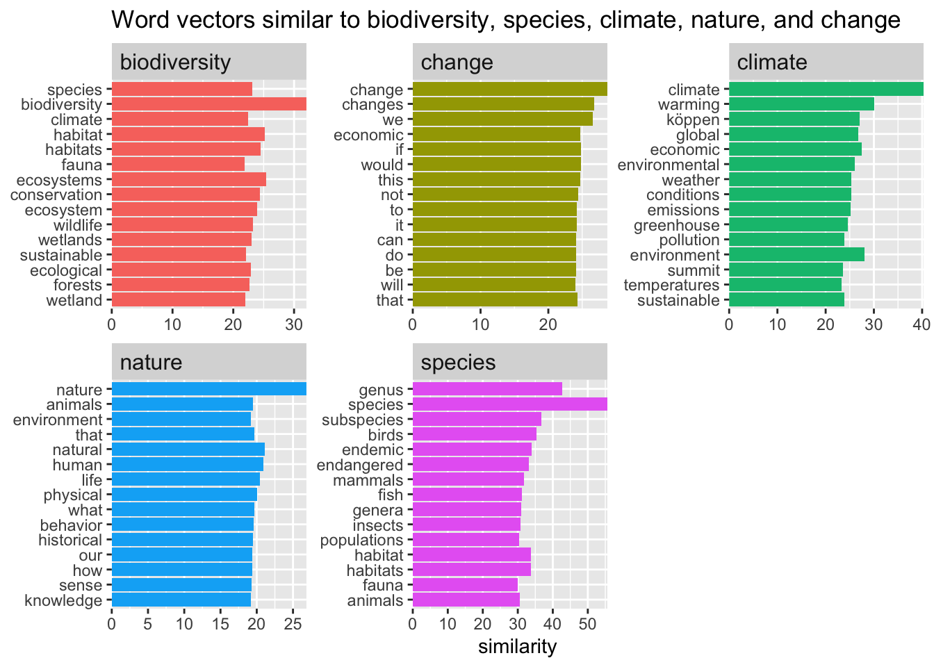
We can recreate our earlier analyses using the GloVe embeddings in places of the embeddings we trained.

The synonym similarities for the GloVe embeddings are much higher than for the articles I selected. The synonyms chosen are also much more pertinent to each word. This is expected since the GloVe embeddings are much more comprehensive.

biodiversity <- search_synonyms(word_vectors = glove6b_matrix, glove6b_matrix['biodiversity',])
biodiversity

# A tibble: 400,000 × 2
   token        similarity
   <chr>             <dbl>
 1 biodiversity       32.0
 2 ecosystems         25.4
 3 habitat            25.2
 4 habitats           24.5
 5 conservation       24.4
 6 ecosystem          24.0
 7 wildlife           23.3
 8 species            23.1
 9 wetlands           23.0
10 ecological         22.9
# … with 399,990 more rows

climate <- search_synonyms(word_vectors = glove6b_matrix, glove6b_matrix['climate',])
climate

# A tibble: 400,000 × 2
   token         similarity
   <chr>              <dbl>
 1 climate             40.4
 2 warming             30.0
 3 environment         28.1
 4 economic            27.5
 5 köppen              27.0
 6 global              26.7
 7 environmental       26.0
 8 weather             25.4
 9 conditions          25.3
10 emissions           25.1
# … with 399,990 more rows

species <- search_synonyms(word_vectors = glove6b_matrix, glove6b_matrix["species",])
species

# A tibble: 400,000 × 2
   token      similarity
   <chr>           <dbl>
 1 species          55.6
 2 genus            42.6
 3 subspecies       36.8
 4 birds            35.3
 5 endemic          34.0
 6 habitat          33.8
 7 habitats         33.8
 8 endangered       33.2
 9 mammals          31.7
10 fish             31.1
# … with 399,990 more rows

nature <- search_synonyms(word_vectors = glove6b_matrix, glove6b_matrix['nature',])
nature

# A tibble: 400,000 × 2
   token      similarity
   <chr>           <dbl>
 1 nature           26.9
 2 natural          21.1
 3 human            20.9
 4 life             20.5
 5 physical         20.1
 6 that             19.7
 7 what             19.6
 8 behavior         19.6
 9 animals          19.5
10 historical       19.4
# … with 399,990 more rows

change <- search_synonyms(word_vectors = glove6b_matrix, glove6b_matrix["change",])
change

# A tibble: 400,000 × 2
   token    similarity
   <chr>         <dbl>
 1 change         28.7
 2 changes        26.7
 3 we             26.5
 4 if             24.9
 5 would          24.8
 6 this           24.7
 7 economic       24.7
 8 not            24.4
 9 that           24.3
10 to             24.2
# … with 399,990 more rows

biodiversity %>%
    mutate(selected = "biodiversity") %>%
    bind_rows(species %>%
                  mutate(selected = "species"),
              climate |> mutate(selected = "climate"),
              nature |> mutate(selected = "nature"),
              change |> mutate(selected = "change")) %>%
    group_by(selected) %>%
    top_n(15, similarity) %>%
    ungroup %>%
    mutate(token = reorder(token, similarity)) %>%
    ggplot(aes(token, similarity, fill = selected)) +
    geom_col(show.legend = FALSE) +
    facet_wrap(~selected, scales = "free") +
    coord_flip() +
    theme(strip.text=element_text(hjust=0, size=12)) +
    scale_y_continuous(expand = c(0,0)) +
    labs(x = NULL, title = "Word vectors similar to biodiversity, species, climate, nature, and change ")

climate_crisis <- glove6b_matrix["climate",] + glove6b_matrix["crisis",]
search_synonyms(glove6b_matrix, climate_crisis)

# A tibble: 400,000 × 2
   token       similarity
   <chr>            <dbl>
 1 climate           61.4
 2 crisis            60.9
 3 economic          60.0
 4 global            53.3
 5 economy           50.4
 6 warming           47.6
 7 situation         46.1
 8 summit            45.6
 9 countries         45.4
10 environment       45.2
# … with 399,990 more rows

no_extinction <- glove6b_matrix["extinction",] - glove6b_matrix["species",]
search_synonyms(glove6b_matrix, no_extinction)

# A tibble: 400,000 × 2
   token              similarity
   <chr>                   <dbl>
 1 non-families             16.1
 2 iyanla                   14.9
 3 (813)                    14.8
 4 meh                      14.5
 5 soundview                14.2
 6 blogs.tampabay.com       14.0
 7 naroff                   13.6
 8 bihn                     13.5
 9 smallcap                 13.3
10 mahagonny                13.1
# … with 399,990 more rows

biodiversity_hotspot <- glove6b_matrix["biodiversity",] + glove6b_matrix["hotspots",]
search_synonyms(glove6b_matrix, biodiversity_hotspot)

# A tibble: 400,000 × 2
   token           similarity
   <chr>                <dbl>
 1 biodiversity          43.9
 2 hotspots              36.4
 3 ecosystems            34.9
 4 habitats              34.3
 5 desertification       32.6
 6 climate               31.0
 7 habitat               30.6
 8 wildlife              30.5
 9 ecosystem             30.4
10 wetlands              30.3
# … with 399,990 more rows