Predicting dissolved inorganic carbon (DIC) concentrations using different algorithms in Python and R

Python

This project uses ocean chemistry data collected by CalCOFI to predict DIC using Linear Regression, KNN, Decision Trees, Random Forest Regressor, Gradient Boosting, and a Support Vector Machine.

Author

Affiliation

Andrew Bartnik

Master of Environmental Data Science Program @ The Bren School (UCSB)

Published

March 18, 2023

Introduction and Background

In this post we will be using chemistry data from seawater collected by the California Cooperative Oceanic Fisheries Investigation (CalCOFI). We will be using temperature, salinity, pH, and other chemical parameters to predict Dissolved Inorganic Carbon (DIC) concentrations. Samples are collected at CalCOFI sampling stations. We will be using different regression models to find which does the best job at predicting DIC. Our models are as follows: Linear Regression (including Ridge and Lasso penalties), K-Nearest Neighbors, Decision Trees, Bagged Decision Trees, Random Forests, Gradient Boosting, and a Support Vector Machine. We will be building each of these models in both Python and R using sklearn and tidymodels, and we will discuss how each of these models work. This is an expansion on an assignment from Machine Learning for Environmental Science as part of the University of California Santa Barbara’s Bren School of the Environment & Management Master of Environmental Data Science (MEDS) Program.

The full list of our predictors are below:

NO2uM - Micromoles of Nitrite per liter of seawater
NO3uM - Micromoles of Nitrate per liter of seawater
NH3uM - Micromoles of Ammonia per liter of seawater
R_TEMP - Reported (Potential) Temperature Celsius
R_Depth - Reported Depth (from pressure, meters)
R_Sal - Reported Salinity (from Specific Volume Anomoly, M³/Kg)
R_DYNHT - Reported Dynamic Height in units of dynamic meters (work per unit mass)
R_Nuts - Reported Ammonium concentration
R_Oxy_micromol - Reported Oxygen concentration micromoles/kilogram
PO4uM - Micromoles of Phosphate per liter of seawater
SiO3uM - Micromoles of Silicate per liter of seawater
TA1 - Total Alkalinity micromoles per kilogram solution
Salinity1 - Salinity (Practical Scale - 1978)
Temperature_degC - Temp (C)

First, we import our required libraries in both languages. We use the reticulate package in R to allow us to execute python code in a quarto doc.

R
Python

library(tidyverse)
library(tidymodels)
library(gridExtra)
library(doParallel)
library(rsample)
library(glmnet)
library(tmap)
library(sf)
library(leaflet)
library(reticulate)
library(baguette)
library(corrplot)

use_condaenv("oceanchem", required = TRUE)

# numpy and pandas for data manipulation + processing
import pandas as pd
import numpy as np

# sklearn and xgboost for our modeling
import xgboost
import sklearn
from sklearn.model_selection import train_test_split, StratifiedKFold, GridSearchCV
from sklearn.linear_model import LinearRegression, Ridge, Lasso
from sklearn.metrics import mean_squared_error
from sklearn.neighbors import KNeighborsRegressor
from sklearn.preprocessing import StandardScaler
from sklearn.pipeline import Pipeline
from sklearn.tree import DecisionTreeRegressor, plot_tree
from sklearn.ensemble import BaggingRegressor
from sklearn.ensemble import RandomForestRegressor
from sklearn.ensemble import GradientBoostingRegressor
from xgboost import XGBRegressor
from sklearn.svm import SVR

# cartopy, matplotlib for plots
from mpl_toolkits.axes_grid1 import make_axes_locatable
from cartopy.mpl.ticker import LongitudeFormatter, LatitudeFormatter
import seaborn as sns
import matplotlib.pyplot as plt
import cartopy.crs as ccrs
import cartopy.feature as cfeature
import plotly

Preprocessing

First, we are going to do some pre-processing and data exploration. The process is essentially the same in both R and python. We first import the data, and make sure our columns are consistent. The actual DIC values for our test set are stored in a separate dataframe, so we’ll also join these onto the test set.

Python
R

We first use pandas to read in our data, merge our solutions to our test set, and make some minor adjustments to column names to ensure consistency.

# Reading in the data using pandas. Join the solutions onto the test set
train_py = pd.read_csv("train.csv")
sols = pd.read_csv("solution.csv")
test_py = pd.read_csv("test.csv")

test_py = pd.merge(test_py, sols, on="id", suffixes=("", "_actual"))
# Dropping the initial index column, renaming TA1 to a more appropriate format
test_py = test_py.drop(test_py.columns[0], axis=1).rename(columns={"TA1.x": "TA1.x"})
train_py = train_py.drop([train_py.columns[0], train_py.columns[12]], axis=1).rename(columns={"TA1.x": "TA1"})

# We will be clearing our environment consistently using the del function in python, just to stay organized and clear up space
del(sols)

Lets plot the data to get a feel for where off the California coast the samples were collected. We’re going to use the cartopy package:


# First, we set up the plot with cartopy
fig = plt.figure(figsize=(10, 10))
ax = fig.add_subplot(1, 1, 1, projection=ccrs.PlateCarree()) # specifying the map projection we want to use

# Next, we'll define the region of interest (California coast)
lat_min, lat_max = 30, 37
lon_min, lon_max = -130, -114

# Set the plot extent (latitude and longitude range of the coast)
ax.set_extent([lon_min, lon_max, lat_min, lat_max])

# Add higher resolution coastlines, land, and ocean features for aesthetics
ax.add_feature(cfeature.NaturalEarthFeature('physical', 'land', '10m', edgecolor='face', facecolor=cfeature.COLORS['land']))
ax.add_feature(cfeature.NaturalEarthFeature('physical', 'ocean', '10m', edgecolor='face', facecolor=cfeature.COLORS['water'], alpha = 0.5))
ax.coastlines(resolution='10m')

# Add the borders of the coastline
ax.add_feature(cfeature.BORDERS, linestyle=':')

# Plot the sampling points 
ax.scatter(train_py['Lon_Dec'], train_py['Lat_Dec'], color='red', marker='o')

# Add labels and title
ax.set_xticks(np.arange(lon_min, lon_max + 1, 2), crs=ccrs.PlateCarree())
ax.set_yticks(np.arange(lat_min, lat_max + 1, 2), crs=ccrs.PlateCarree())
ax.xaxis.set_major_formatter(LongitudeFormatter())
ax.yaxis.set_major_formatter(LatitudeFormatter())
plt.xlabel("Longitude")
plt.ylabel("Latitude")
plt.title("CalCOFI Sampling Points along the California Coast")

plt.show()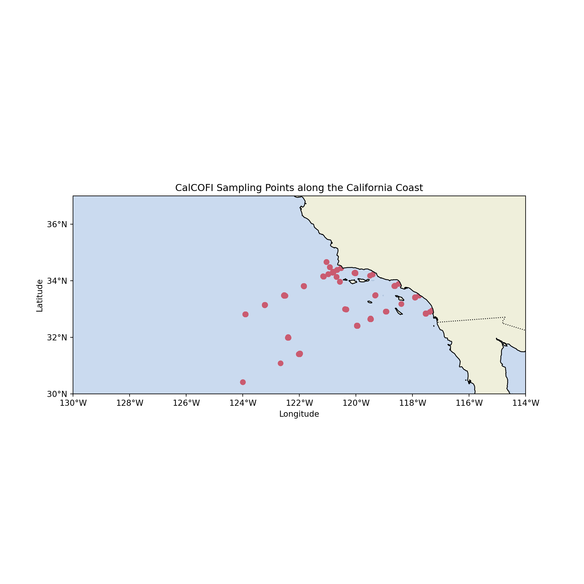

We read in the data the same way in R. We use an inner_join to bind the test values to the dataframe, and filter out the columns that we’re not interested in.

# Read in the solutions data
solutions <- read_csv("solution.csv")
# Read in the testing data, join it to our solutions dataframe. 
testing <- read_csv("test.csv") |> inner_join(solutions, by = "id", suffix = c("", "_actual")) |> select(-1, TA1.x = TA1)

# Read in the training data, getting rid of the redundant id column and the other blank column
training <- read_csv("train.csv") |> select(-1, -...13)

# Using doParallel to specify the number of cores that we want to use for some of our more computationally intensive models.  We'll come back to this later
n_cores <- detectCores() - 1 

# Clearing our environment
rm(solutions)

## Using a corrplot to visualize correlations between our variables
training_cor <- cor(training)
corrplot(training_cor, method = "color")

Our corrplot shows that there are strong correlations between DIC and some of our other variables. Specifically, DIC looks to be highly correlated with Micromoles of Nitrate per liter of seawater, Temperature, Salinity, and a few others.

We can also plot the data in R, instead using leaflet to add some basic interactivity.

# Create a color palette for DIC. This adds another dimension to the data, and we'll be able to clearly see if there is any sort of spatial pattern with DIC
color_palette <- colorNumeric(palette = "YlOrRd", domain = training$DIC)

# Create the leaflet map
leaflet(training) %>%
  addProviderTiles("Esri.WorldImagery", group = "Satellite") %>%
  addProviderTiles("OpenStreetMap", group = "Street Map") %>%
  addCircleMarkers(lng = ~Lon_Dec, lat = ~Lat_Dec,
                   fillColor = ~color_palette(DIC),
                   fillOpacity = 1, stroke = FALSE,
                   radius = 3, group = "Data") %>%
  addLegend(pal = color_palette, values = ~DIC,
            title = "DIC", position = "bottomright") %>%
  addLayersControl(baseGroups = c("Satellite", "Street Map"),
                   overlayGroups = "Data",
                   options = layersControlOptions(collapsed = FALSE))

rm(color_palette)

This was partially an exercise to see if DIC was correlated with distance from the coastline at all, which it doesn’t appear to be.

Feature Engineering

Now we’re going to do some feature engineering. Feature engineering transforms existing data into new data, and helps improve our model performance by capturing relationships that might not be explicit in the data as it is. There are different types of feature engineering, but we’re going to focus on using interaction terms. Interaction terms are used to capture the combined effect of two or more variables on our target variable, DIC. This is particularly important in our context because ocean chemistry is complicated, and we would like to use our domain knowledge to capture some of the relationships between our predictors.

For example, consider the relationship between depth R_Depth and salinity R_Sal. The interaction between depth and salinity can be explained by the fact that as water depth increases, pressure also increases, which affects the solubility of gases in seawater. Salinity also affects the solubility of gases in seawater, so the combined effect of depth and salinity may impact dissolved inorganic carbon levels.

Using this same approach, we are going to include interaction terms for temperature/salinity, and depth/temperature.

Python
R

In Python, we name the new interaction column and set it equal to the product of the terms we want to interact. We repeat this process for each interaction term.

# Adding interaction terms to our training set
train_py['T_degC_Salnty'] = train_py['Temperature_degC'] * train_py['Salinity1']
train_py['Depth_Sal'] = train_py['R_Depth'] * train_py['R_Sal']
train_py['Depth_Temp'] = train_py['R_Depth'] * train_py['Temperature_degC']

# Same thing for the test set
test_py['T_degC_Salnty'] = test_py['Temperature_degC'] * test_py['Salinity1']
test_py['Depth_Sal'] = test_py['R_Depth'] * test_py['R_Sal']
test_py['Depth_Temp'] = test_py['R_Depth'] * test_py['Temperature_degC']

We then make our training and testing objects. We split off DIC and assign it to the y_test and y_train variables below. This allows us to explicitly tell our models which columns we’re using as features, and the outcome we want to predict.

# Splitting off DIC in the training data
X_train = train_py.drop(columns=['DIC'])
y_train = train_py['DIC']

# Same thing for the test data
X_test = test_py.drop(columns=['DIC'])
y_test = test_py['DIC']

We can use the same approach to make our interaction terms in R with the $ operator to initialize new columns:

# Adding interaction terms to our training sets
training$T_degC_Salnty <- training$Temperature_degC * training$Salinity1
training$Depth_Sal <- training$R_Depth * training$R_Sal
training$Depth_Temp <- training$R_Depth * training$Temperature_degC

# Adding interaction terms to our test sets
testing$T_degC_Salnty <- testing$Temperature_degC * testing$Salinity1
testing$Depth_Sal <- testing$R_Depth * testing$R_Sal
testing$Depth_Temp <- testing$R_Depth * testing$Temperature_degC

In R, the tidymodels package provides us with useful functions for splitting training and testing data. We stratify on DIC to ensure that our data is not disproportionately split on the outcome variable, which would bias our model. We also specify our cross-validation parameters using 5 folds, and create a recipe object that we will use throughout our analysis. This recipe object uses our specifications to normalize the numeric variables, and we will use this in each R model. We will also normalize in Python, using pipelines that we create separately for each model.

# Creating 5-fold CV
folds <- vfold_cv(data = training, v = 5, strata = DIC)

# Creating our recipe object
rec <- recipe(DIC ~ ., data = training) |> 
  step_normalize(all_numeric(), -DIC) |> 
  prep()

Linear Regression

Linear regression is the simplest model we can use to make predictions. It is an extremely powerful yet elegant technique used to model the relationship between one or more independent variables (predictors) and dependent variables (features). The basic form of the model is:

\[\operatorname{Y}=\beta_0+\beta_1 x +\beta_n x_n + \varepsilon \] Where $\beta_0$ is our intercept, $\beta_1$, $\beta_n$ are the coefficients of our independent variables, and $\varepsilon$ is the difference between the observed values and the values predicted by our model. We’re going to be evaluating our model performance using the Root Mean Squared Error (RMSE) metric which represents the square root of the average squared differences between the predicted values and the actual observed values. This helps us quantify the difference between the predicted values generated by the model and the actual values of the target variable.

We’re also going to try Lasso and Ridge regression here. Both of these follow the same concepts as regular linear regression, but they implement penalties based on slightly different metrics of the cost function. Ridge regression adds an L2 penalty term, which is the squared magnitude of the $\beta$ coefficients. This penalty term is controlled by alpha, and prevents our model from overfitting the training data by shrinking the coefficients towards zero, thus reducing the variance of the model. Lasso on the other hand uses an L1 penalty term on the cost function, which is based on the absolute magnitude of the coefficients. This penalty term is controlled by lambda, and forces some of the coefficients to be exactly zero, eliminating irrelevant features from the model. Both of these may improve our models’ performance.

Python
R

In Python, we first instantiate a linear regression model, fit it on the training data, and then predict on the holdout data.


# instantiate a Linear Regression model
lr_model = LinearRegression()

# fit the model to the training set
lr_model.fit(X_train, y_train)

# Predict on the test set

LinearRegression()

In a Jupyter environment, please rerun this cell to show the HTML representation or trust the notebook.
On GitHub, the HTML representation is unable to render, please try loading this page with nbviewer.org.

y_test_pred_lr = lr_model.predict(X_test)

# Calculate RMSE on our test set
rmse_test_lr = mean_squared_error(y_test, y_test_pred_lr, squared=False)

print(f"RMSE on the test set: {rmse_test_lr:.2f}")

RMSE on the test set: 4.93

An RMSE of 4.93 is not bad at all! Lets take a look at what this actually looks like plotted through our data:

# clear our plot
plt.clf()
# Create a scatter plot of the true DIC values vs predicted DIC values
plt.scatter(y_test, y_test_pred_lr, alpha=0.5)

# Add a diagonal line representing perfect predictions
diagonal_line = np.linspace(min(y_test.min(), y_test_pred_lr.min()),
                            max(y_test.max(), y_test_pred_lr.max()))
plt.plot(diagonal_line, diagonal_line, color='red', linestyle='--', lw=2)

# Add labels, title and RMSE text
plt.xlabel('True DIC values')
plt.ylabel('Predicted DIC values')
plt.title('True vs Predicted DIC values')
plt.text(0.05, 0.95, f'RMSE: {rmse_test_lr:.2f}', transform=plt.gca().transAxes)

# Show the plot
plt.show()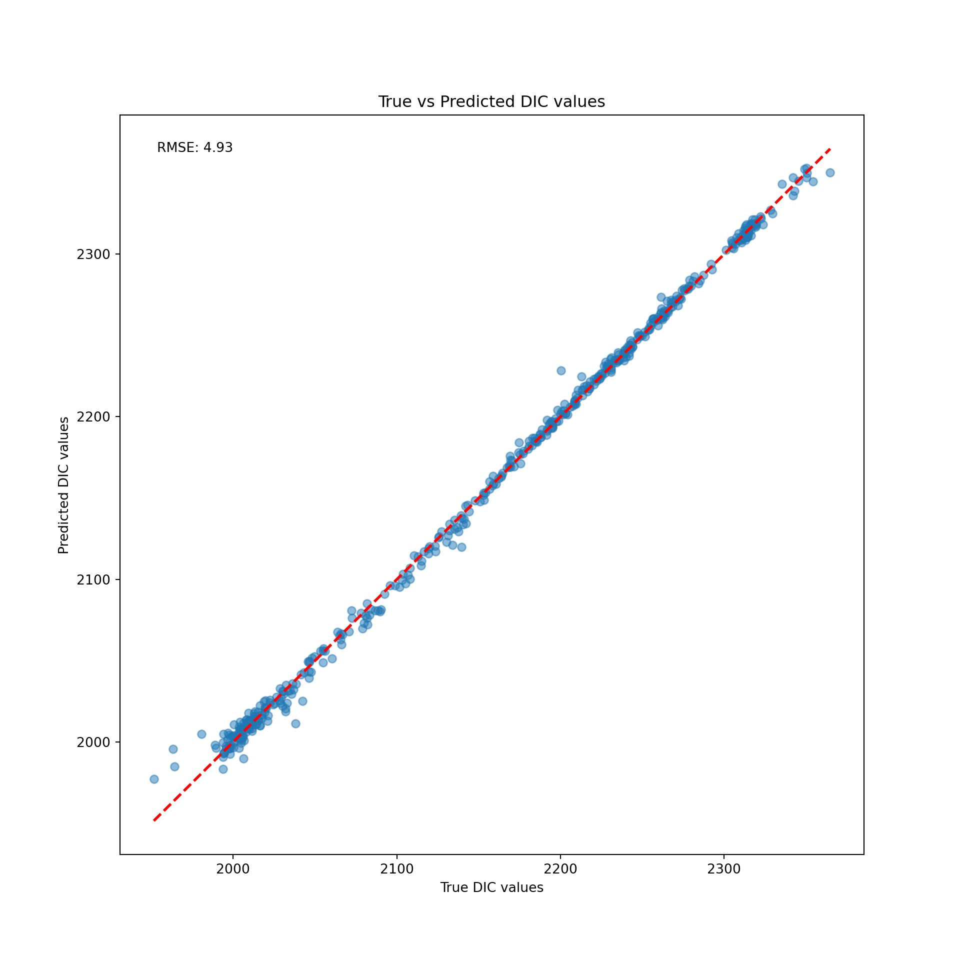

del(lr_model, y_test_pred_lr)

The red line here is what we would have observed if we correctly predicted each observation. The difference between the red line and the blue dots represent the difference between our model’s prediction, and the actual value.

Now we’ll check out Ridge and Lasso regression. We follow the same approach as with linear regression but with one slight change. We specify the alpha parameter, which controls the strength of the penalty. This would usually be a tuning hyperparameter, which I’ll explain in a second, but we’re just going to use an alpha value of one.

plt.clf()

# Ridge Regression
ridge = Ridge(alpha=1)
ridge.fit(X_train, y_train)

Ridge(alpha=1)

ridge_preds = ridge.predict(X_test)
ridge_rmse = mean_squared_error(y_test, ridge_preds, squared=False)
print("Ridge RMSE:", ridge_rmse)

# Lasso Regression

Ridge RMSE: 4.928343737671815

lasso = Lasso(alpha=1)
lasso.fit(X_train, y_train)

Lasso(alpha=1)

lasso_preds = lasso.predict(X_test)
lasso_rmse = mean_squared_error(y_test, lasso_preds, squared=False)
print("Lasso RMSE:", lasso_rmse)

Lasso RMSE: 6.5330738340489605

del(ridge, ridge_preds, lasso, lasso_preds)

While our ridge model achieved a comparable RMSE to our linear regression, our lasso model performed worse. This could be because the lasso model is shrinking important coefficients to zero.

In R, we use our recipe that we defined earlier, then create a linear regression model and a workflow. Our recipe object specifies the preprocessing steps required to transform the data, while the workflow includes both the preprocessing and the modeling steps. We add our recipe and model to our workflow, fit on the training data, and predict on the test data.

# First we create the model
lm_model <- linear_reg() %>%
  set_engine("lm") %>%
  set_mode("regression")


# we then make a workflow, analogous to a pipe in python
lm_workflow <- workflow() |> 
  add_recipe(rec) |> 
  add_model(lm_model)

# fit to training
lm_fit <- fit(lm_workflow, data = training)

# predict on the test data
testing_preds_lr <- predict(lm_fit, testing)

# Calculate and store the RMSE
rmse_test_lr <- rmse(testing_preds_lr, truth = testing$DIC, estimate = .pred)
rmse_lr <- rmse_test_lr$.estimate

print(paste0("RMSE on the holdout set: ", round(rmse_lr, 3)))

[1] "RMSE on the holdout set: 4.933"

# Create a scatter plot of the true DIC values vs predicted DIC values
ggplot(testing, aes(x = DIC, y = testing_preds_lr$.pred)) +
  geom_point(alpha = 0.5) +
  geom_abline(slope = 1, intercept = 0, color = "red", linetype = "dashed", size = 1) +
  labs(
    x = "True DIC values",
    y = "Predicted DIC values",
    title = "True vs Predicted DIC values"
  ) +
  annotate("text", x = min(testing$DIC), y = max(testing$DIC), label = paste("RMSE:", round(rmse_lr, 2)), hjust = 0, vjust = 1)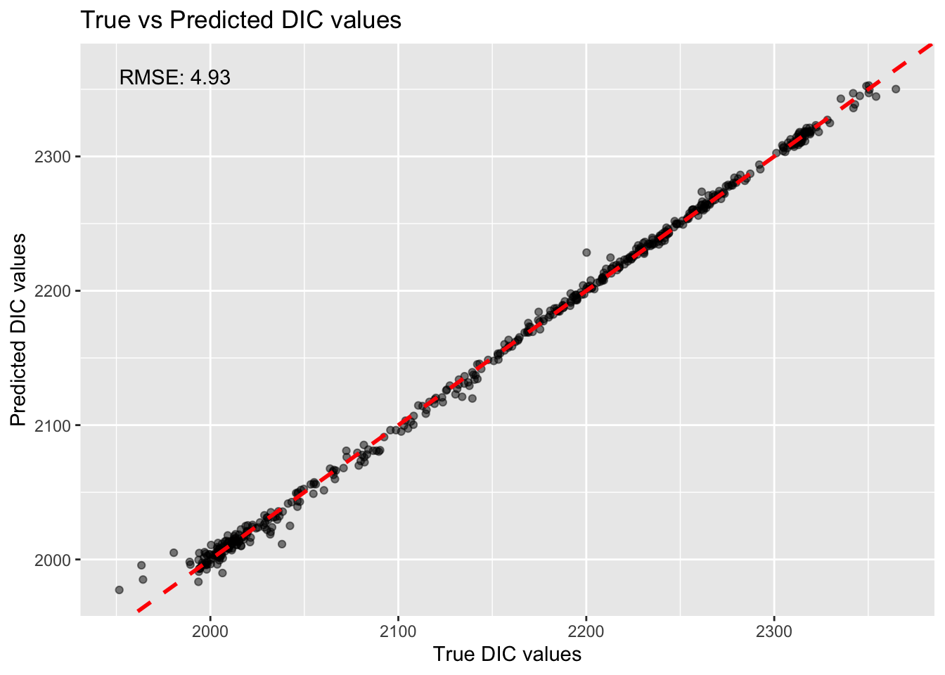

rm(lm_model, lm_workflow, lm_fit, testing_preds_lr, rmse_test_lr)

We achieved a similar RMSE to our linear regression in python, which is reassuring. Now, lets try ridge and lasso penalties in R:

# Ridge Regression, mixture=0 specifies that this is a ridge model
ridge_model <- linear_reg(penalty = 1, mixture = 0) %>%
  set_engine("glmnet") %>%
  set_mode("regression")

# Ridge workflow, add our recipe and model
ridge_workflow <- workflow() |> 
  add_recipe(rec) |> 
  add_model(ridge_model)

# Fit on the training, predict on the test data, store the RMSEs
ridge_fit <- fit(ridge_workflow, data = training)
ridge_testing_preds <- predict(ridge_fit, testing)
ridge_rmse <- as.numeric(rmse(ridge_testing_preds, truth = testing$DIC, estimate = .pred)[,3])
print(paste("Ridge RMSE:", round(ridge_rmse, 2)))

[1] "Ridge RMSE: 7.89"

# Same approach for lasso regression, this time using mixture=1 for lasso
lasso_model <- linear_reg(penalty = 1, mixture = 1) %>%
  set_engine("glmnet") %>%
  set_mode("regression")

# workflow, same as before
lasso_workflow <- workflow() |> 
  add_recipe(rec) |> 
  add_model(lasso_model)
# fit on the training and predict on the test
lasso_fit <- fit(lasso_workflow, data = training)
lasso_testing_preds <- predict(lasso_fit, testing)
lasso_rmse <- as.numeric(rmse(lasso_testing_preds, truth = testing$DIC, estimate = .pred)[,3])
print(paste("Lasso RMSE:", round(lasso_rmse, 2)))

[1] "Lasso RMSE: 5.39"

rm(ridge_model, ridge_workflow, ridge_fit, lasso_model, lasso_workflow, lasso_fit, ridge_testing_preds, lasso_testing_preds)

Both of these models in R performed worse than our regular linear regression model.

Our ridge and lasso models both performed slightly worse than our regular linear regression. This could be because we chose poor values of penalty, which we could address by tuning this hyperparameter. This could also simply be because our penalties might be penalizing coefficients that are actually important for predicting the outcome variable. This can happen when there is high correlation between the predictors. While our Lasso and Ridge models didn’t boost our performance here, they are especially useful for when we have a dataset with a high number of predictors and help us reduce complexity and minimize overfitting.

KNN

The next model we want to try is K-Nearest Neighbors. Usually, this algorithm is used for classification, and would not be my first choice for a regression task. In the context of classification, KNN is used to predict the category of an unknown data point based on the categories of its neighboring data points. Given a scatterplot of data points belonging to different classes (for example, measurements of tree height and leaf width of two distinct species), the algorithm considers a specified number of the closest points (neighbors) to the unknown data point. The unknown point is then assigned a category based on the majority class of these neighbors. KNN can also be applied to regression tasks, where the goal is to predict a continuous value instead of a discrete category. Here, the algorithm again looks at the specified number of nearest neighbors to the unknown data point. However, instead of determining the majority class, it computes the average of the target values of these neighbors. The unknown point is then assigned this average value as its prediction.

We are also tuning our first hyperparameter here: the number of neighbors we want to use. We’re going to use grid searching to find the optimal k, essentially making a grid of a range of values that we expect our optimal value for k to fall within. We search over this grid, test each of the values, and find the value that performs best on the training set. It is important to find the right k-value, as too small of a k will result in overfitting while too large of a k will result in underfitting. We will be using this approach with all models going forward.

Python
R

We follow a slightly different workflow to our linear regression model in python now that we have a tuning parameter. We instantiate the model, specify the number of neighbors we want to test (typically the square root of the total number of observations in the dataset is a good rule of thumb)

# Instantiate our knn regressor
knn_regressor = KNeighborsRegressor()

# Define the parameter grid for hyperparameter tuning - we want to test all numbers of n_neighbors from 1 to 34
param_grid = {'knn__n_neighbors': list(range(1, 35))}

# Create a pipeline with StandardScaler and KNeighborsRegressor
knn_pipeline = Pipeline([
    ('scaler', StandardScaler()),
    ('knn', knn_regressor)
])

# Perform GridSearchCV for hyperparameter tuning
grid_search = GridSearchCV(knn_pipeline, param_grid, cv=5, scoring='neg_root_mean_squared_error')

# fit on the training
grid_search.fit(X_train, y_train)

GridSearchCV(cv=5,
             estimator=Pipeline(steps=[('scaler', StandardScaler()),
                                       ('knn', KNeighborsRegressor())]),
             param_grid={'knn__n_neighbors': [1, 2, 3, 4, 5, 6, 7, 8, 9, 10, 11,
                                              12, 13, 14, 15, 16, 17, 18, 19,
                                              20, 21, 22, 23, 24, 25, 26, 27,
                                              28, 29, 30, ...]},
             scoring='neg_root_mean_squared_error')

We can take a look at how our RMSE changes with different values of k:

# first, clear the figure
plt.clf()
# Get the mean cross-validated scores for each n_neighbors
cv_scores = grid_search.cv_results_['mean_test_score']  

cv_scores = -cv_scores

# Plot RMSE vs. n_neighbors
plt.figure(figsize=(8, 6))
plt.plot(list(range(1, 35)), cv_scores, marker='o')
plt.xlabel('Number of Neighbors (n_neighbors)')
plt.ylabel('Mean Cross-Validated RMSE')
plt.title('RMSE vs. n_neighbors')
plt.grid()
plt.show()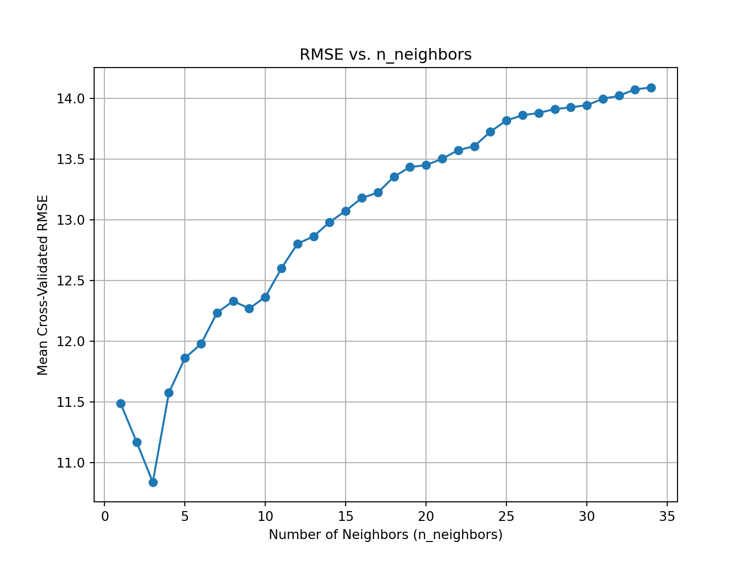

It looks like our best value for k is 3.

# fit on the training
grid_search.fit(X_train, y_train)

# Retrieve the best KNN model

GridSearchCV(cv=5,
             estimator=Pipeline(steps=[('scaler', StandardScaler()),
                                       ('knn', KNeighborsRegressor())]),
             param_grid={'knn__n_neighbors': [1, 2, 3, 4, 5, 6, 7, 8, 9, 10, 11,
                                              12, 13, 14, 15, 16, 17, 18, 19,
                                              20, 21, 22, 23, 24, 25, 26, 27,
                                              28, 29, 30, ...]},
             scoring='neg_root_mean_squared_error')

best_knn = grid_search.best_estimator_

# predict on the test set
y_pred = grid_search.predict(X_test)

# get our RMSE
rmse_knn = mean_squared_error(y_test, y_pred, squared=False)

print("Root Mean Squared Error: ", rmse_knn)

Root Mean Squared Error:  11.332377692549752

del(knn_regressor, param_grid, grid_search, best_knn, y_pred)

RMSE is noticeably worse than our regularized and ordinary linear regression models.

We follow the same approach in R, this time specifying in the model specification that we want to tune the number of neighbors. We make a grid of possible values for our number of neighbors parameter, find the optimal value, then use this value to fit on the training and predict on the test set.

# Make our model
knn_spec <- nearest_neighbor(neighbors = tune()) |> 
  set_engine("kknn") |> 
  set_mode("regression")

# Create a grid
k_grid <- grid_regular(
  neighbors(range = c(1, 34)),
  levels = 30
)

# make our workflow
knn_workflow <- workflow() |> 
  add_model(knn_spec) |> 
  add_recipe(rec)

# tune it!
knn_tuned <- tune_grid(
  knn_workflow,
  resamples = folds,
  grid = k_grid,
  metrics = metric_set(rmse)
)

# Get our optimal value for k
best_k <- knn_tuned |> 
  collect_metrics() |> 
  filter(.metric == "rmse") |> 
  arrange(mean) |> 
  slice(1) |> 
  pull(neighbors)

We can also check how our RMSE changes with different values of our n_neighbors hyperparameter in R.

# Get the RMSE for each n_neighbors from the tuning results
knn_tuning_metrics <- knn_tuned |> 
  collect_metrics() |> 
  filter(.metric == "rmse")

# Plot RMSE vs. n_neighbors
ggplot(knn_tuning_metrics, aes(x = neighbors, y = mean)) +
  geom_point() +
  geom_line() +
  theme_minimal() +
  labs(
    title = "RMSE vs. n_neighbors",
    x = "Number of Neighbors (n_neighbors)",
    y = "Mean Cross-Validated RMSE"
  ) +
  theme(plot.title = element_text(hjust = 0.5))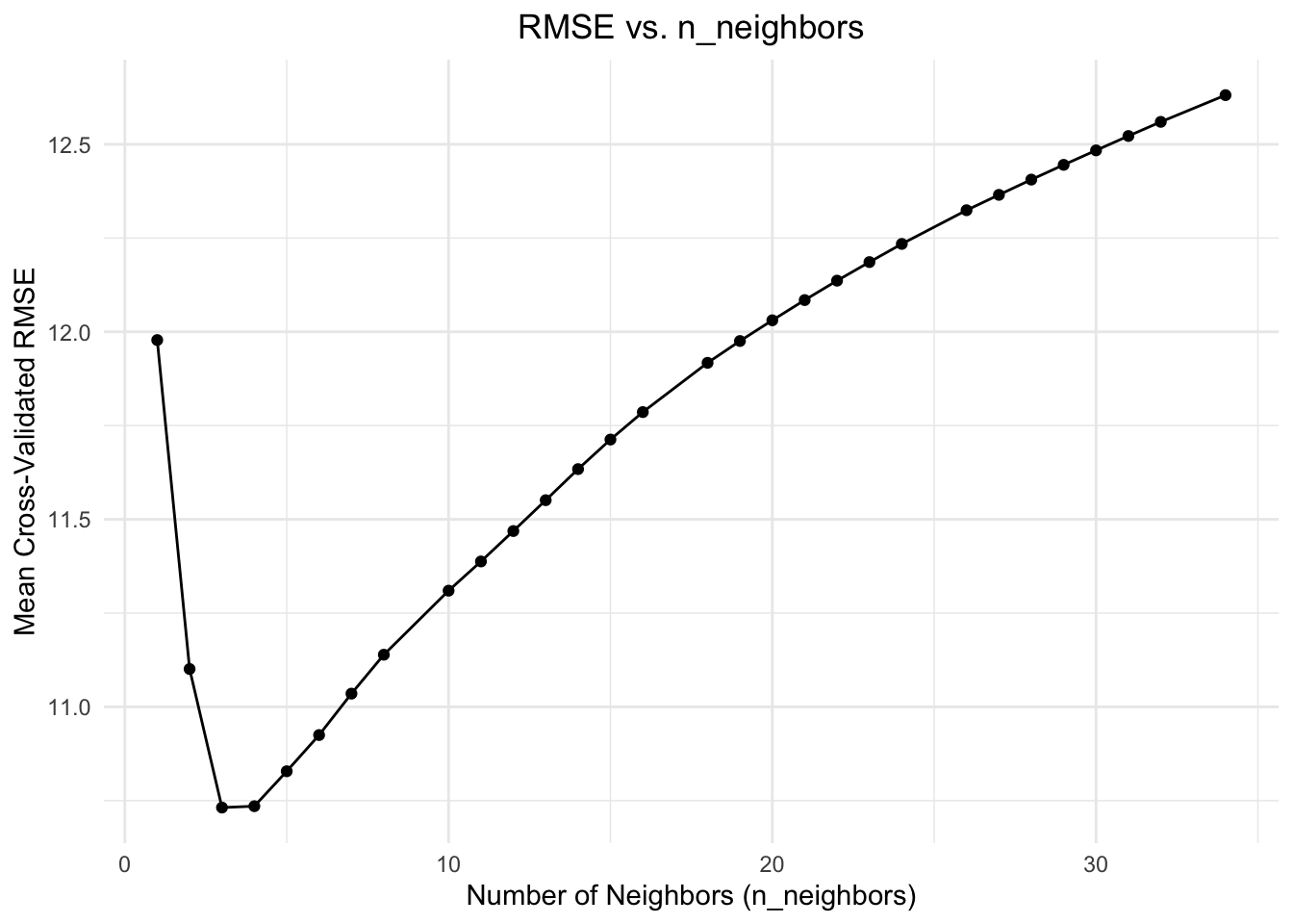

Our best value for K looks to be 5 in R.

# Update our model using our best k
knn_spec_best <- nearest_neighbor(neighbors = best_k) |> 
  set_engine("kknn") |> 
  set_mode("regression")

# Fit the final model on the whole training set
knn_final <- knn_workflow |> 
  update_model(knn_spec_best) |> 
  fit(data = training)

# Make predictions on the test set
knn_testing_preds <- predict(knn_final, testing) |> 
  bind_cols(testing) |> 
  mutate(truth = as.double(DIC), estimate = as.double(.pred)) |> 
  metrics(truth = truth, estimate = estimate)

# RMSE
rmse_knn <- knn_testing_preds |> 
  filter(.metric == "rmse") |> 
  pull(.estimate)

print(paste0("Our KNN RMSE is: ", rmse_knn))

[1] "Our KNN RMSE is: 11.4660152657121"

rm(knn_spec, knn_spec_best, best_k, knn_final, knn_testing_preds, knn_tuned, k_grid, knn_workflow)

Again, our KNN model performs poorly here.

Our RMSE in both of these KNN models were noticeably worse than any of the ordinary linear regression models. No surprises here, this is not a scenario in which we would typically use KNN. Now, we’re going to move on to the tree-based models.

Decision Tree

The next algorithm we’re going to try is the decision tree. Decision trees are a popular algorithm used for both classification and regression tasks. They work by recursively splitting the input data into subsets based on the values of the input features, giving you a tree like structure. Each node in the tree represents a decision rule or condition based on the feature values, while the leaf/terminal nodes represent the final predicted class or value. The process of building a decision tree involves selecting the best feature to split the data at each node, usually based on a criterion such as information gain (for classification) or mean squared error (for regression). The tree continues to grow by making further splits until a stopping criterion is met, such as a minimum number of samples per leaf, a maximum depth of the tree, or a threshold for the improvement in the splitting criterion. A much more comprehensive explanation is here.

Decision trees are great, but can be prone to overfitting. Fortunately, we have hyperparameters to combat this. We’re tuning 3 hyperparameters in this model. The cost complexity penalty, the maximum tree depth, and the minimum leaf samples. The cost complexity is used to “prune” the trees - reducing overfitting by removing branches of the decision tree that do not improve the accuracy of the model. This is similar to our alpha parameter in Lasso/Ridge regression, but penalizes the tree for having too many nodes. The maximum tree depth hyperparameter sets the maximum depth of the decision tree, or the number of levels the tree can have. A deeper tree is more likely to be overfitting the training data. Finally, the minimum number of samples required to be in a leaf node hyperparameter also helps us prevent overfitting and controlling tree depth by requiring a minimum number of samples in each leaf node.

It should be noted, unlike our KNN model, decision trees and their ensembles like random forests and bagged trees are generally not very sensitive to the scale of the input features because they make decisions based on the relative ordering of feature values, rather than the magnitudes of those values. But since we’re using the same recipe object rec for each model in R, all of our features are automatically scaled. We will use the same approach in python, by explicitly creating a Pipeline object with a scaler inside of it for each model.

Python
R

We’re introducting our first pipeline object here. This object is analogous to a workflow in R. We pass it the preprocessing steps we want to use on our data, and our model. We fit this pipeline object to the training data, and predict on the test data.


# Create a pipeline with a scaler and the decision tree regressor
pipe = Pipeline([
    ('scaler', StandardScaler()),
    ('dt_regressor', DecisionTreeRegressor(random_state=4))
])

# Define the parameter grid for hyperparameter tuning
param_grid = {
    'dt_regressor__ccp_alpha': np.logspace(-4, 0, 20), # np.logspace(-4, 0, 5)
    'dt_regressor__max_depth': list(range(1, 13)), # list(range(1, 21))
    'dt_regressor__min_samples_leaf': list(range(1, 13)) # list(range(1, 21))
}

# Perform GridSearchCV for hyperparameter tuning using the pipeline
grid_search = GridSearchCV(pipe, param_grid, cv=5, scoring='neg_root_mean_squared_error', n_jobs=-1)
grid_search.fit(X_train, y_train)

GridSearchCV(cv=5,
             estimator=Pipeline(steps=[('scaler', StandardScaler()),
                                       ('dt_regressor',
                                        DecisionTreeRegressor(random_state=4))]),
             n_jobs=-1,
             param_grid={'dt_regressor__ccp_alpha': array([1.00000000e-04, 1.62377674e-04, 2.63665090e-04, 4.28133240e-04,
       6.95192796e-04, 1.12883789e-03, 1.83298071e-03, 2.97635144e-03,
       4.83293024e-03, 7.84759970e-03, 1.27427499e-02, 2.06913808e-02,
       3.35981829e-02, 5.45559478e-02, 8.85866790e-02, 1.43844989e-01,
       2.33572147e-01, 3.79269019e-01, 6.15848211e-01, 1.00000000e+00]),
                         'dt_regressor__max_depth': [1, 2, 3, 4, 5, 6, 7, 8, 9,
                                                     10, 11, 12],
                         'dt_regressor__min_samples_leaf': [1, 2, 3, 4, 5, 6, 7,
                                                            8, 9, 10, 11, 12]},
             scoring='neg_root_mean_squared_error')

# Make predictions and evaluate the model
y_pred = grid_search.predict(X_test)
dt_rmse = mean_squared_error(y_test, y_pred, squared=False)
print("Best Decision Tree parameters: ", grid_search.best_params_)

Best Decision Tree parameters:  {'dt_regressor__ccp_alpha': 0.03359818286283781, 'dt_regressor__max_depth': 11, 'dt_regressor__min_samples_leaf': 5}

print("RMSE: ", dt_rmse)


# Clear our environment

RMSE:  6.711271577254955

del(pipe, param_grid, grid_search, y_pred)

Our RMSE for this decision tree algorithm is 6.7. Much better than the KNN regressor!

We follow the same approach as we did for KNN in R. We specify the parameters we want to tune in the model specification, make a grid of values to try, and select the best values for our final model.

# decision tree model specification, specifying our hyperparameters to tune. 
dt_spec <- decision_tree(
    mode = "regression",
    cost_complexity = tune(),
    tree_depth = tune(),
    min_n = tune()
  ) |> 
  set_engine("rpart") |> 
  set_mode("regression")

# Define the parameter grid for hyperparameter tuning
param_grid <- grid_regular(cost_complexity(), tree_depth(), min_n(), levels = 5)

# workflow
dt_workflow <- workflow() |> 
  add_model(dt_spec) |> 
  add_recipe(rec)


# tune our parameters
registerDoParallel(cores = n_cores)
dt_tuned <- tune_grid(
  dt_workflow,
  resamples = folds,
  grid = param_grid,
  metrics = metric_set(rmse),
  control = control_grid(save_pred = TRUE, parallel_over = "everything")
)

# extract the best values
best_params <- dt_tuned |> 
  show_best("rmse") |> 
  slice(1) |> 
  select(cost_complexity, tree_depth, min_n) 

best_cc <- best_params$cost_complexity
best_depth <- best_params$tree_depth
best_min_n <- best_params$min_n

print(paste0("Best cost complexity parameter: ", best_cc))

[1] "Best cost complexity parameter: 1e-10"

print(paste0("Best maximum tree depth: ", best_depth))

[1] "Best maximum tree depth: 11"

print(paste0("Best minimum number of samples in a leaf: ", best_min_n))

[1] "Best minimum number of samples in a leaf: 21"

We can also use this autoplot function to visualize our best hyperparameter combinations:

autoplot(dt_tuned)

We now use these best values in our final model:

# Create the final decision tree model with the best hyperparameters
dt_final <- decision_tree(
  cost_complexity = best_cc,
  tree_depth = best_depth,
  min_n = best_min_n
) |> 
  set_engine("rpart") |> 
  set_mode("regression")


# fit to the training
dt_final_fit <- dt_workflow |> 
  update_model(dt_final) |> 
  fit(data = training)

# predict on the test set
dt_testing_preds <- predict(dt_final_fit, testing) |> 
  bind_cols(testing) |> 
  mutate(truth = as.double(DIC), estimate = as.double(.pred)) |> 
  metrics(truth = truth, estimate = estimate)

dt_rmse <- dt_testing_preds |>  filter(.metric == "rmse") |>  pull(.estimate)

print(best_params)

# A tibble: 1 × 3
  cost_complexity tree_depth min_n
            <dbl>      <int> <int>
1    0.0000000001         11    21

print(paste0("RMSE:", dt_rmse))

[1] "RMSE:6.74550963199777"

rm(dt_testing_preds, dt_tuned, dt_final_fit, dt_final, dt_spec, best_params, dt_workflow)

Again, our decision tree in R performs much better than the KNN algorithm we used.

The decision tree model will be the foundation for the next 3 models we are going to try. Bagged Trees, Random Forests, and Gradient Boosting all use decision trees as their base learner, but with slight adjustments to how the final model is constructed.

Bagged Trees

Our normal decision tree algorithm worked well, but there are some significant improvements we can make to this algorithm. Bagging, or bootstrap aggregation is a technique that creates multiple models and then combines their predictions into a final output. Bootstrapping involves drawing samples from a dataset with replacement, to create new samples that are of the same size as the original dataset. By generating multiple samples of the data and predict the statistic of interest for each sample, we can aggregate these predictions into a final output that typically generalizes to unseen data much better than a model trained on a single dataset.

In the context of decision trees, this is an ensemble method that employs the bagging technique by training multiple decision trees on different subsets of the training data. In our case, the new predictions are made by averaging the predictions together from the individual base learners. This technique works particularly well on decision trees, since single decision trees are high variance learners. We’re creating multiple decision trees on different subsets of the training data. Our model’s stability and robustness are increased since the predictions are less sensitive to small changes in the training data. In other words, the variance of the model is reduced, which greatly helps us with avoiding overfitting. Bagged Trees also provide information about the importance of each feature in the model, because each tree is trained on a random subset of the features. This means that each tree will give different weights to different features, which can then be used to identify the most important ones.

We have an additional hyperparameter to train here: the number of trees we want to generate the final bagged model from. Aside from this, the code is much the same as regular decision trees.

Python
R

We specify the n_estimators parameter here to be 500.


# create a pipeline with a scaler and the bagged decision tree model
pipe = Pipeline([
    ('scaler', StandardScaler()),
    ('bagged_dt', BaggingRegressor(estimator=DecisionTreeRegressor(random_state=4), n_estimators=50, random_state=4)) #500
])

# define our grid
param_grid = {
    'bagged_dt__estimator__ccp_alpha': np.logspace(-4, 0, 5), # np.logspace(-4, 0, 20),
    'bagged_dt__estimator__max_depth': list(range(1, 13)), # list(range(1, 21)),
    'bagged_dt__estimator__min_samples_leaf': list(range(1, 13)) # list(range(1, 21))
}

# now lets search our grid for our optimal values
grid_search = GridSearchCV(pipe, param_grid, cv=5, scoring='neg_root_mean_squared_error', n_jobs=-1)
grid_search.fit(X_train, y_train)

GridSearchCV(cv=5,
             estimator=Pipeline(steps=[('scaler', StandardScaler()),
                                       ('bagged_dt',
                                        BaggingRegressor(estimator=DecisionTreeRegressor(random_state=4),
                                                         n_estimators=50,
                                                         random_state=4))]),
             n_jobs=-1,
             param_grid={'bagged_dt__estimator__ccp_alpha': array([1.e-04, 1.e-03, 1.e-02, 1.e-01, 1.e+00]),
                         'bagged_dt__estimator__max_depth': [1, 2, 3, 4, 5, 6,
                                                             7, 8, 9, 10, 11,
                                                             12],
                         'bagged_dt__estimator__min_samples_leaf': [1, 2, 3, 4,
                                                                    5, 6, 7, 8,
                                                                    9, 10, 11,
                                                                    12]},
             scoring='neg_root_mean_squared_error')

# predict on the test set
y_pred = grid_search.predict(X_test)
bag_tree_rmse = mean_squared_error(y_test, y_pred, squared=False)
print("Best Bagged Decision Tree parameters: ", grid_search.best_params_)

Best Bagged Decision Tree parameters:  {'bagged_dt__estimator__ccp_alpha': 0.001, 'bagged_dt__estimator__max_depth': 12, 'bagged_dt__estimator__min_samples_leaf': 2}

print("Bagged Decision Tree RMSE: ", bag_tree_rmse)

Bagged Decision Tree RMSE:  4.996459665683262

del(pipe, param_grid, grid_search, y_pred)

Our RMSE is improving!

As usual, we follow the same approach in R. We specify the number of trees we want to use in the final model using times=500.

# model specification
bagdt_spec <- bag_tree(
    mode = "regression",
    tree_depth = tune(),
    min_n = tune(),
    cost_complexity = tune()
  ) %>%
  set_engine("rpart", times = 50) |> # times = 500
  set_mode("regression")

# checking out our hyperparameters
bagdt_params <- parameters(cost_complexity(), tree_depth(), min_n())
bagdt_grid <- grid_max_entropy(bagdt_params, size = 10, iter = 5)

# make a workflow
bagdt_wf <- workflow() |>
  add_model(bagdt_spec) |>
  add_recipe(rec)

# Tuning
n_cores <- detectCores() - 1 # Use all available cores except one
registerDoParallel(cores = n_cores)
bagdt_rs <- tune_grid(
  bagdt_wf,
  resamples = folds,
  grid = bagdt_grid,
  metrics = metric_set(yardstick::rmse),
  control = control_grid(save_pred = TRUE, parallel_over = "everything")
)

# Get the best hyperparameters
best_bagdt_params <- bagdt_rs |> 
  show_best("rmse") |> 
  slice(1) |> 
  select(cost_complexity, tree_depth, min_n)

best_cc_bagdt <- best_bagdt_params$cost_complexity
best_depth_bagdt <- best_bagdt_params$tree_depth
best_min_n_bagdt <- best_bagdt_params$min_n

show_best(bagdt_rs)

# A tibble: 5 × 9
  cost_complexity tree_depth min_n .metric .estima…¹  mean     n std_err .config
            <dbl>      <int> <int> <chr>   <chr>     <dbl> <int>   <dbl> <chr>  
1   0.000000580           12    30 rmse    standard   6.41     5   0.509 Prepro…
2   0.00000000243          8    29 rmse    standard   6.46     5   0.516 Prepro…
3   0.0000460             10     9 rmse    standard   6.67     5   0.477 Prepro…
4   0.0000560             13    24 rmse    standard   6.75     5   0.511 Prepro…
5   0.00000144             5    22 rmse    standard   6.91     5   0.519 Prepro…
# … with abbreviated variable name ¹.estimator

We can again use the handy autoplot() function to visualize our best hyperparameter combinations:

autoplot(bagdt_rs)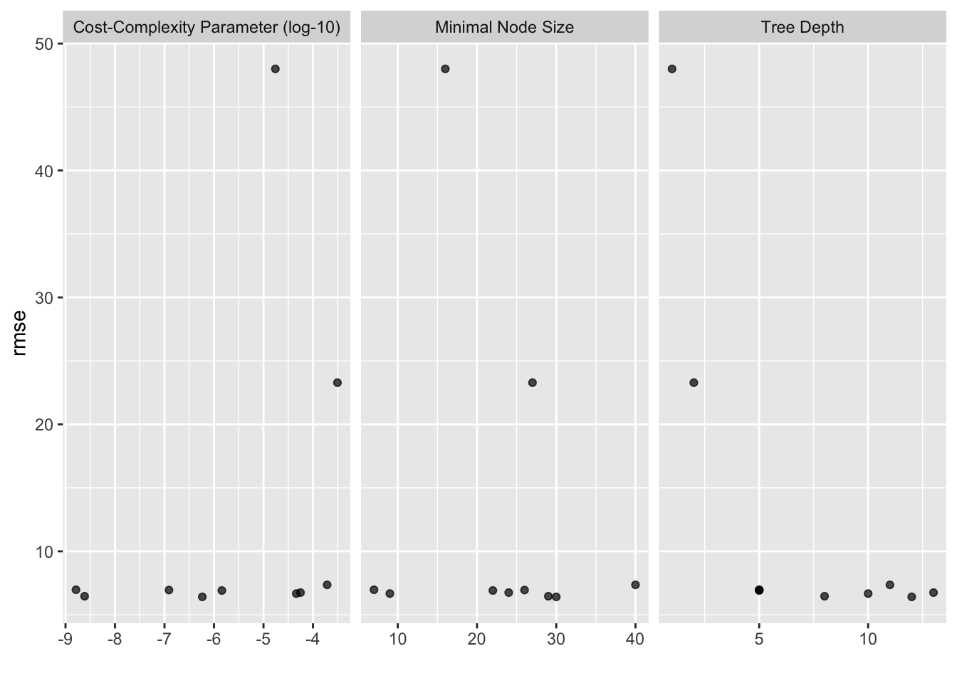

And finally, we use our best hyperparameter values to construct our final model.

# Create the final decision tree model with the best hyperparameters
bagdt_final <- bag_tree(
  cost_complexity = best_cc_bagdt,
  tree_depth = best_depth_bagdt,
  min_n = best_min_n_bagdt
) %>%
  set_engine("rpart") %>%
  set_mode("regression")


# Fit the final model on the whole training set
bagdt_final_fit <- bagdt_wf %>%
  update_model(bagdt_final) %>%
  fit(data = training)

# Make predictions on the holdout set and compute the RMSE
bagdt_testing_preds <- predict(bagdt_final_fit, testing) |> 
  bind_cols(testing) |> 
  mutate(truth = as.double(DIC), estimate = as.double(.pred)) |> 
  metrics(truth = truth, estimate = estimate)

bagdt_rmse <- bagdt_testing_preds %>% filter(.metric == "rmse") |>  pull(.estimate)
print(paste0("Bagged Tree RMSE:", bagdt_rmse))

[1] "Bagged Tree RMSE:5.79701120060714"

rm(bagdt_final, bagdt_final_fit, bagdt_grid, bagdt_params, bagdt_rs, bagdt_spec, bagdt_testing_preds, bagdt_wf, best_bagdt_params)

Our RMSE is getting better! Bagging our decision trees help us combat the overfitting that ordinary decision trees are prone to. However, there are still a few more ways we can improve this model!

Random Forest

Our Bagged Tree RMSE was better than our normal decision tree algorithm, but we can still make this better! Bagging aggregates the predictions across all the trees, which reduces the variance of the overall procedure and results in improved predictive performance. However, simply bagging trees results in tree correlation that limits the effect of variance reduction. Random forests are built using the same fundamental principles as decision trees and bagging, but inject further randomness in the process which further reduces the variance.

Random forests help to reduce tree correlation by injecting more randomness into the tree-growing process. Specifically, while growing a decision tree during the bagging process, random forests specify a subset of the features to be used in each tree. This parameter is called m_try, and it controls the number of features to consider when randomly selecting a subset of features for each tree. For example, if there are 10 input features and mtry is set to 3, then for each tree in the Random Forest, a random subset of 3 features will be selected from the 10 input features. By controlling the number of features used for each tree, mtry helps to reduce the correlation between the trees and increase the diversity of the Random Forest. The optimal value for m_try depends on the problem, but a standard value for regression tasks ismtry=(p/3), where p is the number of features present in our dataset.

Python
R

# Create a pipeline with a scaler and the random forest regressor
pipe = Pipeline([
    ('scaler', StandardScaler()),
    ('rf_regressor', RandomForestRegressor(random_state=4))
])

# Define the parameter grid for hyperparameter tuning
param_grid = {
    'rf_regressor__n_estimators': list(range(100, 1000, 50)),  
    'rf_regressor__max_features': list(range(1, X_train.shape[1] - 10)),  # mtry
    'rf_regressor__min_samples_leaf': list(range(1, 10))  # min_n
}

# Perform GridSearchCV for hyperparameter tuning
grid_search = GridSearchCV(pipe, param_grid, cv=5, scoring='neg_root_mean_squared_error', n_jobs=-1)
grid_search.fit(X_train, y_train)

# Make predictions and evaluate the model

GridSearchCV(cv=5,
             estimator=Pipeline(steps=[('scaler', StandardScaler()),
                                       ('rf_regressor',
                                        RandomForestRegressor(random_state=4))]),
             n_jobs=-1,
             param_grid={'rf_regressor__max_features': [1, 2, 3, 4, 5, 6, 7, 8],
                         'rf_regressor__min_samples_leaf': [1, 2, 3, 4, 5, 6, 7,
                                                            8, 9],
                         'rf_regressor__n_estimators': [100, 150, 200, 250, 300,
                                                        350, 400, 450, 500, 550,
                                                        600, 650, 700, 750, 800,
                                                        850, 900, 950]},
             scoring='neg_root_mean_squared_error')

y_pred = grid_search.predict(X_test)
rf_rmse = mean_squared_error(y_test, y_pred, squared=False)
print("Best Random Forest parameters: ", grid_search.best_params_)

Best Random Forest parameters:  {'rf_regressor__max_features': 6, 'rf_regressor__min_samples_leaf': 1, 'rf_regressor__n_estimators': 950}

print("RMSE: ", rf_rmse)

# Clear our environment

RMSE:  5.0701395088877605

del(pipe, param_grid, grid_search, y_pred)

Our RMSE is still improving!

We follow the same approach in R:

# specifying tuning parameters
randfor_spec <- rand_forest(
  trees = tune(),
  mtry = tune(),
  min_n = tune()
) |>
  set_mode("regression") |>
  set_engine("ranger")

# Looking at hyperparameters
randf_grid <-grid_regular(trees(), min_n(), mtry(range(1:13)), levels = 5)

# Define new workflow
rf_workflow <- workflow() |>
  add_model(randfor_spec) |>
  add_recipe(rec)

# Tuning
doParallel::registerDoParallel()
randf_rs <- tune_grid(
  rf_workflow,
  resamples = folds,
  grid = randf_grid,
  metrics = metric_set(yardstick::rmse),
  control = control_grid(save_pred = TRUE, parallel_over = "everything")
)

As always, lets take a look at our best hyperparameter combinations:

autoplot(randf_rs)

# Get the best hyperparameters
best_randf_params <- randf_rs |> 
  show_best("rmse") |> 
  slice(1) |> 
  select(trees, mtry, min_n)

best_trees_rf <- best_randf_params$trees
best_mtry_rf <- best_randf_params$mtry
best_min_n_rf <- best_randf_params$min_n

show_best(randf_rs)

# A tibble: 5 × 9
   mtry trees min_n .metric .estimator  mean     n std_err .config              
  <int> <int> <int> <chr>   <chr>      <dbl> <int>   <dbl> <chr>                
1     7   500     2 rmse    standard    5.74     5   0.497 Preprocessor1_Model0…
2     7  2000     2 rmse    standard    5.75     5   0.497 Preprocessor1_Model0…
3     7  1500     2 rmse    standard    5.76     5   0.490 Preprocessor1_Model0…
4     7  1000     2 rmse    standard    5.77     5   0.505 Preprocessor1_Model0…
5     4  1000     2 rmse    standard    5.78     5   0.436 Preprocessor1_Model0…

# Create the final random forest model with the best hyperparameters
randf_final <- rand_forest(
  trees = best_trees_rf,
  mtry = best_mtry_rf,
  min_n = best_min_n_rf
) |>
  set_mode("regression") |>
  set_engine("ranger")


# fit on the training
randf_final_fit <- rf_workflow |> 
  update_model(randf_final) |> 
  fit(data = training)

# predict on the test, calculate RMSE
rf_testing_preds <- predict(randf_final_fit, testing) |> 
  bind_cols(testing) |> 
  mutate(truth = as.double(DIC), estimate = as.double(.pred)) |> 
  metrics(truth = truth, estimate = estimate)

rf_rmse <- rf_testing_preds %>% filter(.metric == "rmse") |>  pull(.estimate)

rm(randf_grid, randf_rs, randfor_spec, rf_workflow)
print(paste0("Random Forest RMSE:", rf_rmse))

[1] "Random Forest RMSE:5.11937341919548"

Our model is still improving, but there is another powerful adjustment we can make to it.

Gradient Boosting

Whereas random forests build an ensemble of deep independent trees, Gradient Boosting Machines (GBMS) build an ensemble of shallow trees in sequence, with each tree learning and improving on the previous one. Independently, these trees are relatively weak predictive models, but they can be boosted to produce a powerful ensemble of trees.

The boosting idea is to add new models to the ensemble sequentially. We start with a weak model, and sequentially boost its performance by continuing to build new trees, where each new tree in the sequence remedies where the previous one made had the largest prediction errors. To quantify the amount of information gained by each new tree, we use a loss function, which measures the difference between the predicted values and the true values for the training examples. The goal is to minimize this function, which means that we want to find the set of parameters for each new tree that best fit the data. To find the optimal set of parameters, we use gradient descent, which is an optimization algorithm that works by iteratively improving the parameters of the model to minimize the loss function. At each iteration, we calculate the gradient of the loss function with respect to the model parameters, and we use this gradient to update the parameters in a direction that minimizes the loss function. We continue this process until we reach a minimum value of the loss function or a stopping criterion is met. The important hyperparameter we use for this is known as the learning rate. The learning rate specifies how fast we want to descend down the gradient. Too large, and we might miss the minimum of the loss function. Too small, and we’ll need to many iterations to find the minimum.

We’re going to take a different approach to tuning this model. Instead of specifying all the parameters we want to tune in one step, we’re going to break it up. First, we’ll find the optimal learning rate. Based off the optimal learning rate, we’ll then tune the tree specific parameters (min_n/xgb__min_child_weight, tree_depth/xgb__max_depth, loss_reduction/xgb__gamma, xgb__n_estimators in python, we’ll set the number of trees manually in R). Then, based off these optimal values of the tree specific parameters, we’ll tune the stochastic parameters (sample_size/xgb__subsample, mtry/xgb__colsample_bytree).

Python
R

Instead of using sklearn for this algorithm in python, we’re going to use the XGB library. This is a library built specifically for gradient boosting, and will increase our computational efficiency.

# instantiate our GBM
xgb = XGBRegressor()

# make our pipeline
pipeline = Pipeline([
    ('scaler', StandardScaler()),
    ('xgb', xgb)
])
# First, tune the learning rate
learning_rates = np.linspace(0.01, 0.6, 50) # np.linspace(0.01, 0.6, 100)
param_grid_learning_rate = {
    'xgb__learning_rate': learning_rates
}

grid_search_lr = GridSearchCV(
    pipeline, param_grid_learning_rate, cv=5, scoring='neg_root_mean_squared_error', n_jobs=-1
)
grid_search_lr.fit(X_train, y_train)

GridSearchCV(cv=5,
             estimator=Pipeline(steps=[('scaler', StandardScaler()),
                                       ('xgb',
                                        XGBRegressor(base_score=None,
                                                     booster=None,
                                                     callbacks=None,
                                                     colsample_bylevel=None,
                                                     colsample_bynode=None,
                                                     colsample_bytree=None,
                                                     early_stopping_rounds=None,
                                                     enable_categorical=False,
                                                     eval_metric=None,
                                                     feature_types=None,
                                                     gamma=None, gpu_id=None,
                                                     grow_policy=None,
                                                     importance_type=Non...
       0.25081633, 0.26285714, 0.27489796, 0.28693878, 0.29897959,
       0.31102041, 0.32306122, 0.33510204, 0.34714286, 0.35918367,
       0.37122449, 0.38326531, 0.39530612, 0.40734694, 0.41938776,
       0.43142857, 0.44346939, 0.4555102 , 0.46755102, 0.47959184,
       0.49163265, 0.50367347, 0.51571429, 0.5277551 , 0.53979592,
       0.55183673, 0.56387755, 0.57591837, 0.58795918, 0.6       ])},
             scoring='neg_root_mean_squared_error')

GridSearchCV

GridSearchCV(cv=5,
             estimator=Pipeline(steps=[('scaler', StandardScaler()),
                                       ('xgb',
                                        XGBRegressor(base_score=None,
                                                     booster=None,
                                                     callbacks=None,
                                                     colsample_bylevel=None,
                                                     colsample_bynode=None,
                                                     colsample_bytree=None,
                                                     early_stopping_rounds=None,
                                                     enable_categorical=False,
                                                     eval_metric=None,
                                                     feature_types=None,
                                                     gamma=None, gpu_id=None,
                                                     grow_policy=None,
                                                     importance_type=Non...
       0.25081633, 0.26285714, 0.27489796, 0.28693878, 0.29897959,
       0.31102041, 0.32306122, 0.33510204, 0.34714286, 0.35918367,
       0.37122449, 0.38326531, 0.39530612, 0.40734694, 0.41938776,
       0.43142857, 0.44346939, 0.4555102 , 0.46755102, 0.47959184,
       0.49163265, 0.50367347, 0.51571429, 0.5277551 , 0.53979592,
       0.55183673, 0.56387755, 0.57591837, 0.58795918, 0.6       ])},
             scoring='neg_root_mean_squared_error')

estimator: Pipeline

Pipeline(steps=[('scaler', StandardScaler()),
                ('xgb',
                 XGBRegressor(base_score=None, booster=None, callbacks=None,
                              colsample_bylevel=None, colsample_bynode=None,
                              colsample_bytree=None, early_stopping_rounds=None,
                              enable_categorical=False, eval_metric=None,
                              feature_types=None, gamma=None, gpu_id=None,
                              grow_policy=None, importance_type=None,
                              interaction_constraints=None, learning_rate=None,
                              max_bin=None, max_cat_threshold=None,
                              max_cat_to_onehot=None, max_delta_step=None,
                              max_depth=None, max_leaves=None,
                              min_child_weight=None, missing=nan,
                              monotone_constraints=None, n_estimators=100,
                              n_jobs=None, num_parallel_tree=None,
                              predictor=None, random_state=None, ...))])

StandardScaler

StandardScaler()

XGBRegressor

XGBRegressor(base_score=None, booster=None, callbacks=None,
             colsample_bylevel=None, colsample_bynode=None,
             colsample_bytree=None, early_stopping_rounds=None,
             enable_categorical=False, eval_metric=None, feature_types=None,
             gamma=None, gpu_id=None, grow_policy=None, importance_type=None,
             interaction_constraints=None, learning_rate=None, max_bin=None,
             max_cat_threshold=None, max_cat_to_onehot=None,
             max_delta_step=None, max_depth=None, max_leaves=None,
             min_child_weight=None, missing=nan, monotone_constraints=None,
             n_estimators=100, n_jobs=None, num_parallel_tree=None,
             predictor=None, random_state=None, ...)

best_learning_rate = grid_search_lr.best_params_['xgb__learning_rate']
print(f"Best learning rate: {best_learning_rate}")

Best learning rate: 0.3351020408163265

Now, with our best learning rate, we’ll tune the tree-specific parameters. Note that the names of these hyperparameters have changed slightly since we’re using a different package.

# Tree-specific parameters
param_grid_tree = {
    'xgb__min_child_weight': range(1, 10, 3), # range(1, 21, 1),
    'xgb__max_depth': range(1, 10, 3), # range(1, 21, 1),
    'xgb__gamma': np.linspace(0, 1, 5), # np.linspace(0, 1, 20),
    'xgb__n_estimators': range(100, 1500, 700)  # adjust the number of trees np.linspace(100, 1500, 30) 
}

# Set the learning rate 
pipeline.set_params(xgb__learning_rate=best_learning_rate)

# find our best tree-specific parameters

Pipeline(steps=[('scaler', StandardScaler()),
                ('xgb',
                 XGBRegressor(base_score=None, booster=None, callbacks=None,
                              colsample_bylevel=None, colsample_bynode=None,
                              colsample_bytree=None, early_stopping_rounds=None,
                              enable_categorical=False, eval_metric=None,
                              feature_types=None, gamma=None, gpu_id=None,
                              grow_policy=None, importance_type=None,
                              interaction_constraints=None,
                              learning_rate=0.3351020408163265, max_bin=None,
                              max_cat_threshold=None, max_cat_to_onehot=None,
                              max_delta_step=None, max_depth=None,
                              max_leaves=None, min_child_weight=None,
                              missing=nan, monotone_constraints=None,
                              n_estimators=100, n_jobs=None,
                              num_parallel_tree=None, predictor=None,
                              random_state=None, ...))])

grid_search_tree = GridSearchCV(
    pipeline, param_grid_tree, cv=5, scoring='neg_root_mean_squared_error', n_jobs=-1
)
grid_search_tree.fit(X_train, y_train)

# Get the best tree-specific parameters

GridSearchCV(cv=5,
             estimator=Pipeline(steps=[('scaler', StandardScaler()),
                                       ('xgb',
                                        XGBRegressor(base_score=None,
                                                     booster=None,
                                                     callbacks=None,
                                                     colsample_bylevel=None,
                                                     colsample_bynode=None,
                                                     colsample_bytree=None,
                                                     early_stopping_rounds=None,
                                                     enable_categorical=False,
                                                     eval_metric=None,
                                                     feature_types=None,
                                                     gamma=None, gpu_id=None,
                                                     grow_policy=None,
                                                     importance_type=Non...
                                                     min_child_weight=None,
                                                     missing=nan,
                                                     monotone_constraints=None,
                                                     n_estimators=100,
                                                     n_jobs=None,
                                                     num_parallel_tree=None,
                                                     predictor=None,
                                                     random_state=None, ...))]),
             n_jobs=-1,
             param_grid={'xgb__gamma': array([0.  , 0.25, 0.5 , 0.75, 1.  ]),
                         'xgb__max_depth': range(1, 10, 3),
                         'xgb__min_child_weight': range(1, 10, 3),
                         'xgb__n_estimators': range(100, 1500, 700)},
             scoring='neg_root_mean_squared_error')

GridSearchCV

GridSearchCV(cv=5,
             estimator=Pipeline(steps=[('scaler', StandardScaler()),
                                       ('xgb',
                                        XGBRegressor(base_score=None,
                                                     booster=None,
                                                     callbacks=None,
                                                     colsample_bylevel=None,
                                                     colsample_bynode=None,
                                                     colsample_bytree=None,
                                                     early_stopping_rounds=None,
                                                     enable_categorical=False,
                                                     eval_metric=None,
                                                     feature_types=None,
                                                     gamma=None, gpu_id=None,
                                                     grow_policy=None,
                                                     importance_type=Non...
                                                     min_child_weight=None,
                                                     missing=nan,
                                                     monotone_constraints=None,
                                                     n_estimators=100,
                                                     n_jobs=None,
                                                     num_parallel_tree=None,
                                                     predictor=None,
                                                     random_state=None, ...))]),
             n_jobs=-1,
             param_grid={'xgb__gamma': array([0.  , 0.25, 0.5 , 0.75, 1.  ]),
                         'xgb__max_depth': range(1, 10, 3),
                         'xgb__min_child_weight': range(1, 10, 3),
                         'xgb__n_estimators': range(100, 1500, 700)},
             scoring='neg_root_mean_squared_error')

estimator: Pipeline

Pipeline(steps=[('scaler', StandardScaler()),
                ('xgb',
                 XGBRegressor(base_score=None, booster=None, callbacks=None,
                              colsample_bylevel=None, colsample_bynode=None,
                              colsample_bytree=None, early_stopping_rounds=None,
                              enable_categorical=False, eval_metric=None,
                              feature_types=None, gamma=None, gpu_id=None,
                              grow_policy=None, importance_type=None,
                              interaction_constraints=None,
                              learning_rate=0.3351020408163265, max_bin=None,
                              max_cat_threshold=None, max_cat_to_onehot=None,
                              max_delta_step=None, max_depth=None,
                              max_leaves=None, min_child_weight=None,
                              missing=nan, monotone_constraints=None,
                              n_estimators=100, n_jobs=None,
                              num_parallel_tree=None, predictor=None,
                              random_state=None, ...))])

StandardScaler

StandardScaler()

XGBRegressor

XGBRegressor(base_score=None, booster=None, callbacks=None,
             colsample_bylevel=None, colsample_bynode=None,
             colsample_bytree=None, early_stopping_rounds=None,
             enable_categorical=False, eval_metric=None, feature_types=None,
             gamma=None, gpu_id=None, grow_policy=None, importance_type=None,
             interaction_constraints=None, learning_rate=0.3351020408163265,
             max_bin=None, max_cat_threshold=None, max_cat_to_onehot=None,
             max_delta_step=None, max_depth=None, max_leaves=None,
             min_child_weight=None, missing=nan, monotone_constraints=None,
             n_estimators=100, n_jobs=None, num_parallel_tree=None,
             predictor=None, random_state=None, ...)

best_min_child_weight = grid_search_tree.best_params_['xgb__min_child_weight']
best_max_depth = grid_search_tree.best_params_['xgb__max_depth']
best_gamma = grid_search_tree.best_params_['xgb__gamma']
best_n_estimators = grid_search_tree.best_params_['xgb__n_estimators']

print(f"Best min_n: {best_min_child_weight}")

Best min_n: 1

print(f"Best max_depth: {best_max_depth}")

Best max_depth: 4

print(f"Best lost_reduction: {best_gamma}")

Best lost_reduction: 0.25

print(f"Best n_trees: {best_n_estimators}")

Best n_trees: 800

Now that we have the tree-specific parameters tuned, we can move on to the stochastic hyperparameters.

# Stochastic parameters
param_grid_stochastic = {
    'xgb__subsample': np.linspace(0.5, 1, 10), #np.linspace(0.5, 1, 20)
    'xgb__colsample_bytree': np.linspace(1, 15, 15), # np.linspace(1, 15, 15)
}

# Use the best learning rate and tree-specific parameters 
pipeline.set_params(
    xgb__learning_rate=best_learning_rate,
    xgb__min_child_weight=best_min_child_weight,
    xgb__max_depth=best_max_depth,
    xgb__gamma=best_gamma,
    xgb__n_estimators=best_n_estimators
)

# Perform GridSearchCV for stochastic parameters

Pipeline(steps=[('scaler', StandardScaler()),
                ('xgb',
                 XGBRegressor(base_score=None, booster=None, callbacks=None,
                              colsample_bylevel=None, colsample_bynode=None,
                              colsample_bytree=None, early_stopping_rounds=None,
                              enable_categorical=False, eval_metric=None,
                              feature_types=None, gamma=0.25, gpu_id=None,
                              grow_policy=None, importance_type=None,
                              interaction_constraints=None,
                              learning_rate=0.3351020408163265, max_bin=None,
                              max_cat_threshold=None, max_cat_to_onehot=None,
                              max_delta_step=None, max_depth=4, max_leaves=None,
                              min_child_weight=1, missing=nan,
                              monotone_constraints=None, n_estimators=800,
                              n_jobs=None, num_parallel_tree=None,
                              predictor=None, random_state=None, ...))])

grid_search_stochastic = GridSearchCV(
    pipeline, param_grid_stochastic, cv=5, scoring='neg_root_mean_squared_error', n_jobs=-1
)
grid_search_stochastic.fit(X_train, y_train)

# Get the best stochastic parameters

GridSearchCV(cv=5,
             estimator=Pipeline(steps=[('scaler', StandardScaler()),
                                       ('xgb',
                                        XGBRegressor(base_score=None,
                                                     booster=None,
                                                     callbacks=None,
                                                     colsample_bylevel=None,
                                                     colsample_bynode=None,
                                                     colsample_bytree=None,
                                                     early_stopping_rounds=None,
                                                     enable_categorical=False,
                                                     eval_metric=None,
                                                     feature_types=None,
                                                     gamma=0.25, gpu_id=None,
                                                     grow_policy=None,
                                                     importance_type=Non...
                                                     n_estimators=800,
                                                     n_jobs=None,
                                                     num_parallel_tree=None,
                                                     predictor=None,
                                                     random_state=None, ...))]),
             n_jobs=-1,
             param_grid={'xgb__colsample_bytree': array([ 1.,  2.,  3.,  4.,  5.,  6.,  7.,  8.,  9., 10., 11., 12., 13.,
       14., 15.]),
                         'xgb__subsample': array([0.5       , 0.55555556, 0.61111111, 0.66666667, 0.72222222,
       0.77777778, 0.83333333, 0.88888889, 0.94444444, 1.        ])},
             scoring='neg_root_mean_squared_error')

GridSearchCV

GridSearchCV(cv=5,
             estimator=Pipeline(steps=[('scaler', StandardScaler()),
                                       ('xgb',
                                        XGBRegressor(base_score=None,
                                                     booster=None,
                                                     callbacks=None,
                                                     colsample_bylevel=None,
                                                     colsample_bynode=None,
                                                     colsample_bytree=None,
                                                     early_stopping_rounds=None,
                                                     enable_categorical=False,
                                                     eval_metric=None,
                                                     feature_types=None,
                                                     gamma=0.25, gpu_id=None,
                                                     grow_policy=None,
                                                     importance_type=Non...
                                                     n_estimators=800,
                                                     n_jobs=None,
                                                     num_parallel_tree=None,
                                                     predictor=None,
                                                     random_state=None, ...))]),
             n_jobs=-1,
             param_grid={'xgb__colsample_bytree': array([ 1.,  2.,  3.,  4.,  5.,  6.,  7.,  8.,  9., 10., 11., 12., 13.,
       14., 15.]),
                         'xgb__subsample': array([0.5       , 0.55555556, 0.61111111, 0.66666667, 0.72222222,
       0.77777778, 0.83333333, 0.88888889, 0.94444444, 1.        ])},
             scoring='neg_root_mean_squared_error')

estimator: Pipeline

Pipeline(steps=[('scaler', StandardScaler()),
                ('xgb',
                 XGBRegressor(base_score=None, booster=None, callbacks=None,
                              colsample_bylevel=None, colsample_bynode=None,
                              colsample_bytree=None, early_stopping_rounds=None,
                              enable_categorical=False, eval_metric=None,
                              feature_types=None, gamma=0.25, gpu_id=None,
                              grow_policy=None, importance_type=None,
                              interaction_constraints=None,
                              learning_rate=0.3351020408163265, max_bin=None,
                              max_cat_threshold=None, max_cat_to_onehot=None,
                              max_delta_step=None, max_depth=4, max_leaves=None,
                              min_child_weight=1, missing=nan,
                              monotone_constraints=None, n_estimators=800,
                              n_jobs=None, num_parallel_tree=None,
                              predictor=None, random_state=None, ...))])

StandardScaler

StandardScaler()

XGBRegressor

XGBRegressor(base_score=None, booster=None, callbacks=None,
             colsample_bylevel=None, colsample_bynode=None,
             colsample_bytree=None, early_stopping_rounds=None,
             enable_categorical=False, eval_metric=None, feature_types=None,
             gamma=0.25, gpu_id=None, grow_policy=None, importance_type=None,
             interaction_constraints=None, learning_rate=0.3351020408163265,
             max_bin=None, max_cat_threshold=None, max_cat_to_onehot=None,
             max_delta_step=None, max_depth=4, max_leaves=None,
             min_child_weight=1, missing=nan, monotone_constraints=None,
             n_estimators=800, n_jobs=None, num_parallel_tree=None,
             predictor=None, random_state=None, ...)

best_subsample = grid_search_stochastic.best_params_['xgb__subsample']
best_colsample_bytree = grid_search_stochastic.best_params_['xgb__colsample_bytree']

print(f"Best subsample: {best_subsample}")

Best subsample: 1.0

print(f"Best colsample_bytree: {best_colsample_bytree}")

Best colsample_bytree: 1.0

And finally, we can use the best values for all of these hyperparameters to build our final model.

# Train the final model with the best hyperparameters on the training set (excluding the holdout set)
final_pipeline = pipeline.set_params(
    xgb__learning_rate=best_learning_rate,
    xgb__min_child_weight=best_min_child_weight,
    xgb__max_depth=best_max_depth,
    xgb__gamma=best_gamma,
    xgb__n_estimators=best_n_estimators,
    xgb__subsample=best_subsample,
    xgb__colsample_bytree=best_colsample_bytree
)
final_pipeline.fit(X_train, y_train)

# Validate the final model on the holdout set

Pipeline(steps=[('scaler', StandardScaler()),
                ('xgb',
                 XGBRegressor(base_score=None, booster=None, callbacks=None,
                              colsample_bylevel=None, colsample_bynode=None,
                              colsample_bytree=1.0, early_stopping_rounds=None,
                              enable_categorical=False, eval_metric=None,
                              feature_types=None, gamma=0.25, gpu_id=None,
                              grow_policy=None, importance_type=None,
                              interaction_constraints=None,
                              learning_rate=0.3351020408163265, max_bin=None,
                              max_cat_threshold=None, max_cat_to_onehot=None,
                              max_delta_step=None, max_depth=4, max_leaves=None,
                              min_child_weight=1, missing=nan,
                              monotone_constraints=None, n_estimators=800,
                              n_jobs=None, num_parallel_tree=None,
                              predictor=None, random_state=None, ...))])

test_preds = final_pipeline.predict(X_test)
gb_rmse = mean_squared_error(y_test, test_preds, squared=False)
print(f"test RMSE: {gb_rmse}")

test RMSE: 5.038058931912597

Similarly in R, we start by tuning the learning rate. As we have before, we use a grid of values to test to find which produces the lowest RMSE on the training data.

# tune learning rate
tune_lr <- boost_tree(learn_rate = tune()) |> 
  set_mode('regression') |> 
  set_engine("xgboost") 

# make our cv grid
lr_grid <- expand.grid(learn_rate = seq(0.0001, 0.5, length.out = 10)) # seq(0.0001, 0.5, length.out = 200))

# now our workflow
tune_wf_lr <- workflow() |> 
      add_model(tune_lr) |> 
      add_recipe(rec) 

# tuning
fit_tune_lr <- tune_wf_lr |> 
      tune_grid(resamples = folds, grid = lr_grid)

show_best(fit_tune_lr, metric = "rmse")

# A tibble: 5 × 7
  learn_rate .metric .estimator  mean     n std_err .config              
       <dbl> <chr>   <chr>      <dbl> <int>   <dbl> <chr>                
1      0.444 rmse    standard    7.39     5   0.357 Preprocessor1_Model09
2      0.5   rmse    standard    7.95     5   0.308 Preprocessor1_Model10
3      0.389 rmse    standard    8.20     5   0.700 Preprocessor1_Model08
4      0.333 rmse    standard    9.57     5   0.776 Preprocessor1_Model07
5      0.278 rmse    standard   19.2      5   0.365 Preprocessor1_Model06

best_lr <- as.numeric(show_best(fit_tune_lr, metric = "rmse")[1,1])

Using this learning rate, we then tune the tree specific parameters. Unlike our approach in python, we’re fixing the number of trees to be 1000 in R.

registerDoParallel(cores = n_cores)
# Specifying that we want to tune the tree-specific parameters
lropt_tune_spec <-
    boost_tree(
    learn_rate = best_lr,
    trees = 500,
    min_n = tune(),
    tree_depth = tune(),
    loss_reduction = tune()
  ) |>
  set_engine("xgboost") |>
  set_mode('regression')

# Setting up the parameters to be tuned and the grid to search over
tree_params <- parameters(tree_depth(), min_n(), loss_reduction())
trees_grid <- grid_max_entropy(tree_params, size = 5, iter = 2) # size=20

# Defining a new workflow, adding our models and tuning parameters
tree_wf <- workflow() |> add_model(lropt_tune_spec) |> add_recipe(rec)

#  tune our parameters
fit_tune_trees <- tree_wf |> tune_grid(
  resamples = folds,
  grid = trees_grid,
  metrics = metric_set(rmse),
  control = control_grid(save_pred = TRUE, parallel_over = "everything")
)

# extract the best values
show_best(fit_tune_trees, metric ="rmse")

# A tibble: 5 × 9
  min_n tree_depth loss_reduction .metric .estimator  mean     n std_err .config
  <int>      <int>          <dbl> <chr>   <chr>      <dbl> <int>   <dbl> <chr>  
1     4          3       4.49e-10 rmse    standard    6.64     5   0.349 Prepro…
2    13          4       4.79e- 8 rmse    standard    6.88     5   0.313 Prepro…
3    28          4       2.59e-10 rmse    standard    7.06     5   0.374 Prepro…
4    14         11       4.41e- 3 rmse    standard    7.15     5   0.387 Prepro…
5    38         14       7.50e- 8 rmse    standard    7.23     5   0.263 Prepro…

opt_min_n <- as.numeric(show_best(fit_tune_trees, metric = "rmse")[1,1])
opt_tree_depth <- as.numeric(show_best(fit_tune_trees, metric = "rmse")[1,2])
opt_loss_red <- as.numeric(show_best(fit_tune_trees, metric = "rmse")[1,3])

We now use our optimal tree parameters to tune the stochastic parameters.

registerDoParallel(cores = n_cores)

# Specifying that we want to tune the stoachastic-specific parameters
stoch_tune_spec <-
  boost_tree(
    learn_rate = best_lr,
    trees = 500, # 1000
    min_n = opt_min_n,
    tree_depth = opt_tree_depth,
    loss_reduction = opt_loss_red,
    mtry = tune(),
    sample_size = tune()
  ) |>
  set_engine("xgboost") |>
  set_mode('regression')

# Define the parameters
stoch_params <- parameters(
  finalize(mtry(), training),
  sample_size= sample_prop())

# Generate a grid of parameter values
stoch_grid <- grid_max_entropy(stoch_params, size = 5, iter = 2)
        
stoch_tune_wf <- workflow() |> 
  add_model(stoch_tune_spec) |> 
  add_recipe(rec)

fit_tune_stoch <- stoch_tune_wf |> tune_grid(
  resamples = folds,
  grid = stoch_grid,
  metrics = metric_set(rmse),
  control = control_grid(save_pred = TRUE, parallel_over = "everything")
)
show_best(fit_tune_stoch, metric = "rmse")

# A tibble: 5 × 8
   mtry sample_size .metric .estimator  mean     n std_err .config             
  <int>       <dbl> <chr>   <chr>      <dbl> <int>   <dbl> <chr>               
1    18       0.861 rmse    standard    7.20     5   0.353 Preprocessor1_Model2
2    10       0.716 rmse    standard    7.76     5   0.380 Preprocessor1_Model3
3    15       0.468 rmse    standard    8.02     5   0.357 Preprocessor1_Model1
4     7       0.332 rmse    standard   10.2      5   0.455 Preprocessor1_Model5
5    16       0.104 rmse    standard   29.1      5   1.86  Preprocessor1_Model4

opt_mtry <- as.numeric(show_best(fit_tune_stoch, metric = "rmse")[1,1])
opt_ss <- as.numeric(show_best(fit_tune_stoch, metric = "rmse")[1,2])

Finally, we add all of this into the final model

final_model <- boost_tree(learn_rate = best_lr,
                          trees = 500, # 1000
                          min_n = opt_min_n,
                          mtry = opt_mtry,
                          tree_depth = opt_tree_depth,
                          loss_reduction = opt_loss_red,
                          sample_size = opt_ss,
                          ) |>
  set_mode("regression") |>
  set_engine("xgboost", early_stopping_rounds = 10)

final_wf <- workflow() |>
  add_model(final_model) |>
  add_recipe(rec)

final_fit <- final_wf |> fit(training)

# predict on the test, calculate RMSE
gb_testing_preds <- predict(final_fit, testing) |> 
  bind_cols(testing) |> 
  mutate(truth = as.double(DIC), estimate = as.double(.pred)) |> 
  metrics(truth = truth, estimate = estimate)

gb_rmse <- gb_testing_preds %>% filter(.metric == "rmse") |>  pull(.estimate)

print(gb_rmse)

[1] 5.502003

Support Vector Machine

Support Vector Machines (SVMs) are a little different than what we’ve done so far. The goal of SVMs in our case is to move our data into higher dimensions to find a hyperplane that best fits our data points, while balancing model complexity and error tolerance. SVMs accomplish this by transforming the input data into a higher-dimensional space using the kernel trick (implicitly transforming the data into a higher dimensional space without explicitly performing the transformation, this helps the algorithm capture complex relationships in the data without compromising too much computational efficiency). SVMs identify a subset of the training data, called support vectors, which are critical in determining the optimal hyperplane. Once the optimal hyperplane is found, new data points can be projected onto it to make predictions.

The kernel function is what maps the features to a higher-dimensional feature space. Although there are different types of kernel functions to choose from, the linear kernel function is the most appropriate for our data. The linear kernel function is particularly useful when the data is linearly separable or when a linear relationship exists between the features and the target variable.

Python
R

# Create the pipeline
pipe = Pipeline([
    ('scaler', StandardScaler()),
    ('svm', SVR(kernel='linear'))
])

# Define the tuning grid
param_grid = {
    'svm__C': np.logspace(-5, 5, 10), # np.logspace(-5, 5, 100),
}

# Perform grid search with cross-validation
grid = GridSearchCV(pipe, param_grid=param_grid, cv=5, scoring='neg_mean_squared_error', n_jobs=-1)
grid.fit(X_train, y_train)

# Train the final model with the best parameters

GridSearchCV(cv=5,
             estimator=Pipeline(steps=[('scaler', StandardScaler()),
                                       ('svm', SVR(kernel='linear'))]),
             n_jobs=-1,
             param_grid={'svm__C': array([1.00000000e-05, 1.29154967e-04, 1.66810054e-03, 2.15443469e-02,
       2.78255940e-01, 3.59381366e+00, 4.64158883e+01, 5.99484250e+02,
       7.74263683e+03, 1.00000000e+05])},
             scoring='neg_mean_squared_error')

best_params = grid.best_params_
final_model = grid.best_estimator_

# Make predictions on the validation set
y_pred = final_model.predict(X_test)

# Calculate the RMSE
svm_rmse = np.sqrt(mean_squared_error(y_test, y_pred))
print(f"RMSE: {svm_rmse}")

RMSE: 4.8924520113025824

# make our SVM model
svm_model <- svm_linear(
  cost = tune()
) |>
  set_mode("regression") |>
  set_engine("kernlab")

# add model to workflow
svm_workflow <- workflow() |>
  add_model(svm_model) |>
  add_recipe(rec)

# specify our tuning grid
tune_svm_grid <- grid_regular(
  cost(range = c(-10, 10)),
  levels = 5
)

# tune our model
fit_tune_svm <- svm_workflow |>
  tune_grid(
    resamples = folds,
    grid = tune_svm_grid,
    metrics = metric_set(rmse),
    control = control_grid(save_pred = TRUE, parallel_over = "everything")
  )

# extract the best values for the hyperparameters
best_svm_params <- fit_tune_svm |>
  show_best(metric = "rmse") |>
  dplyr::slice(1) |>
  select(cost)

# use our best values in the final model
final_svm_model <- svm_linear(
  cost = best_svm_params$cost
) |>
  set_mode("regression") |>
  set_engine("kernlab")

# make a new workflow
final_svm_wf <- workflow() |>
  add_model(final_svm_model) |>
  add_recipe(rec)

final_svm_fit <- final_svm_wf |> fit(training)

 Setting default kernel parameters

final_svm_pred <- final_svm_fit |> predict(testing)

svm_rmse <- final_svm_pred |>
  bind_cols(testing) |>
  rmse(truth = DIC, estimate = .pred) %>%
  pull(.estimate)

print("RMSE:")

[1] "RMSE:"

print(svm_rmse)

[1] 5.63947

Evaluation

We’ve now finished running our last model. Now, we want to consolidate all of our RMSE scores to compare our different models’ performances. We can easily do this with a bar chart.

Python
R



plt.clf()
model_names = ["LR", "Lasso", "Ridge", "KNN", "DT", "Bag DT", "RF", "GB", "SVM"]
rmses = [rmse_test_lr, ridge_rmse, lasso_rmse, rmse_knn, dt_rmse, bag_tree_rmse, rf_rmse, gb_rmse, svm_rmse]


model_scores = sorted(zip(model_names, rmses), key=lambda x: x[1])
model_names, rmses = zip(*model_scores)

fig, ax = plt.subplots()
ax.bar(model_names, rmses)

<BarContainer object of 9 artists>

ax.set_xlabel("Model")
ax.set_ylabel("RMSE")
ax.set_title("Model Performance Comparison")
plt.xticks(rotation = 45)

([0, 1, 2, 3, 4, 5, 6, 7, 8], [Text(0, 0, 'SVM'), Text(1, 0, 'Lasso'), Text(2, 0, 'LR'), Text(3, 0, 'Bag DT'), Text(4, 0, 'GB'), Text(5, 0, 'RF'), Text(6, 0, 'Ridge'), Text(7, 0, 'DT'), Text(8, 0, 'KNN')])

plt.show()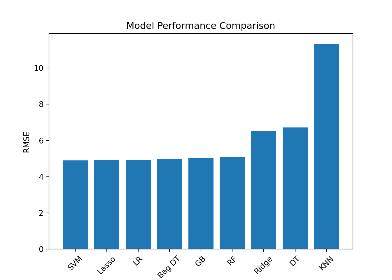

model_names <- c("Linear Regression", "Lasso", "Ridge", "KNN", "Decision Tree", "Bagged DT", "Random Forest", "Gradient Boosting", "SVM")
rmses <- c(rmse_lr, lasso_rmse, ridge_rmse, rmse_knn, dt_rmse, bagdt_rmse, rf_rmse, gb_rmse, svm_rmse)

df_rmse <- data.frame(Model = model_names, RMSE = rmses)
df_rmse <- df_rmse[order(df_rmse$RMSE), ]

ggplot(df_rmse, aes(x = reorder(Model, RMSE), y = RMSE, fill = Model)) +
  geom_bar(stat = "identity") +
  theme(axis.text.x = element_text(angle = 45, hjust = 1)) +
  labs(x = "Model", y = "RMSE", title = "Model Performance Comparison")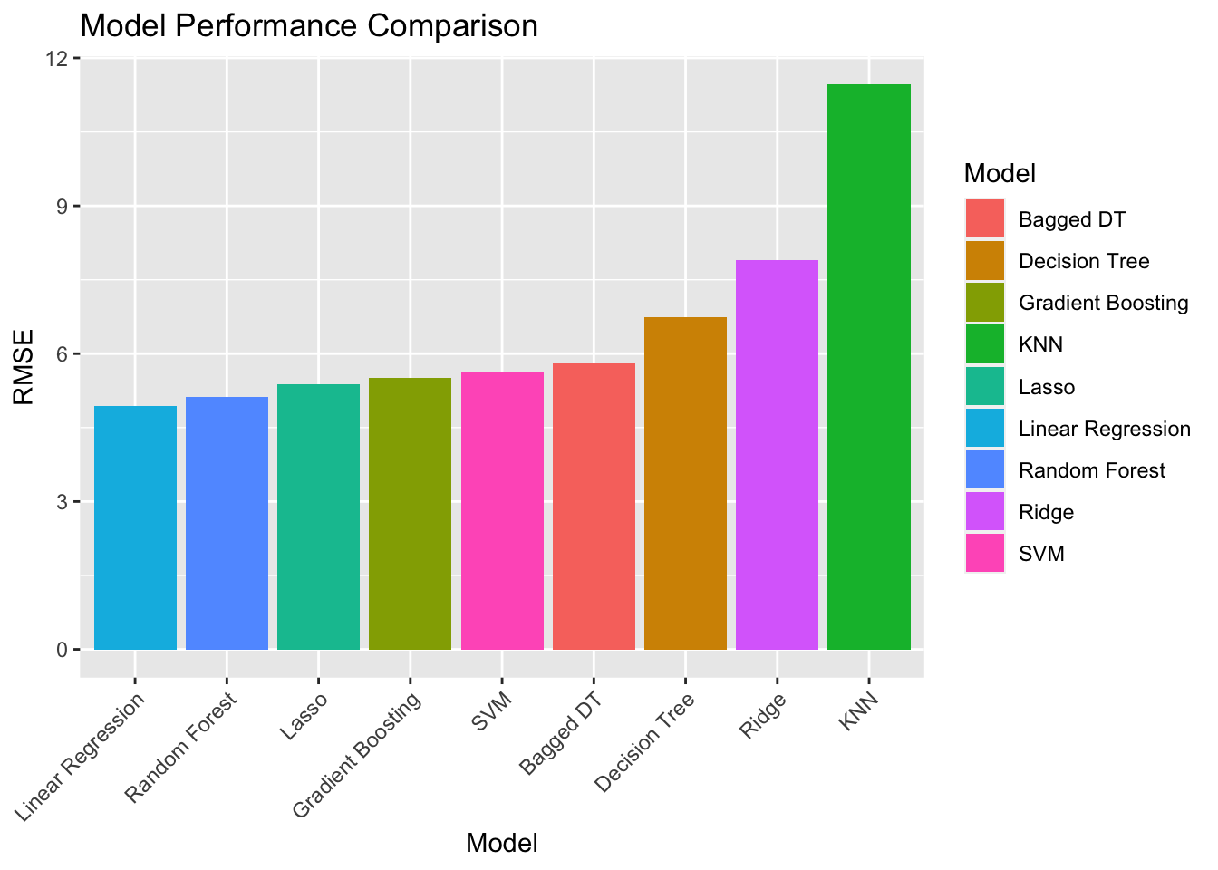

Conclusion

Our SVM model performed the best in Python, while the linear regression performed the best in R. Overall, our linear regression performed consistently well across both languages. This is expected, given that our predictors are highly linearly correlated with the DIC variable. Our random forest regressor and support vector machines also performed quite well, which is sensible since these models also perform well with linearly correlated data. When we tuned our more complicated models (random forest, gradient boosting, svm), we kept the hyperparameter combination grids to search over fairly small. This is because our computation time exponentially increases as we specify more combinations of parameters to search over. This means that the combinations of hyperparameters we searched over may not have had an optimal combination of values, resulting in a lower score. In future work, we could greatly increase the size of the grids to search over, which would probably give us much better performances.

Another thing to note is that while we used RMSE to evaluate our models, this isn’t the only metric that can be used for evaluation, and the best metric depends on the problem. RMSE is a common measure for regression models and is appropriate for our case where we are predicting a continuous variable. In future work, we could explore more feature engineering techniques, or combining our models into an ensemble.

Citation

BibTeX citation:

@online{bartnik2023,
  author = {Andrew Bartnik},
  title = {Predicting Dissolved Inorganic Carbon {(DIC)} Concentrations
    Using Different Algorithms in {Python} and {R}},
  date = {03/18/2023},
  url = {https://andrewbartnik.github.io/Portfolio/ocean-modeling},
  langid = {en}
}

For attribution, please cite this work as:

Andrew Bartnik. 3AD–18AD. “Predicting Dissolved Inorganic Carbon (DIC) Concentrations Using Different Algorithms in Python and R.” 3AD–18AD. https://andrewbartnik.github.io/Portfolio/ocean-modeling.