Analyzing the Effects of the Texas February 2021 Storm on the Houston metropolitan Area

Spatial

Assignments

This post is based on an EDS 223 - Spatial Analysis assignment, as part of the Masters of Environmental Data Science (MEDS) curriculum at the University of California, Santa Barbara’s Bren School of the Environment.

Author

Affiliation

Andrew Bartnik

Master of Environmental Data Science Program @ The Bren School (UCSB)

Published

November 15, 2022

Overview

“In February 2021, the state of Texas suffered a major power crisis, which came about as a result of three severe winter storms sweeping across the United States on February 10–11, 13–17, and 15–20.”¹ For more background, check out these engineering and political perspectives.

We were tasked with:
- estimating the number of homes in Houston that lost power as a result of the first two storms
- investigating if socioeconomic factors are predictors of communities recovery from a power outage

Our analysis was based on remotely-sensed night lights data, acquired from the Visible Infrared Imaging Radiometer Suite (VIIRS) onboard the Suomi satellite. We used VNP46A1 to detect differences in night lights before and after the storm to identify areas that lost electric power.

To determine the number of homes that lost power, we linked (spatially join) these areas with OpenStreetMap data on buildings and roads.

To investigate potential socioeconomic factors that influenced recovery, we linked our analysis with data from the US Census Bureau.

Data

Night lights

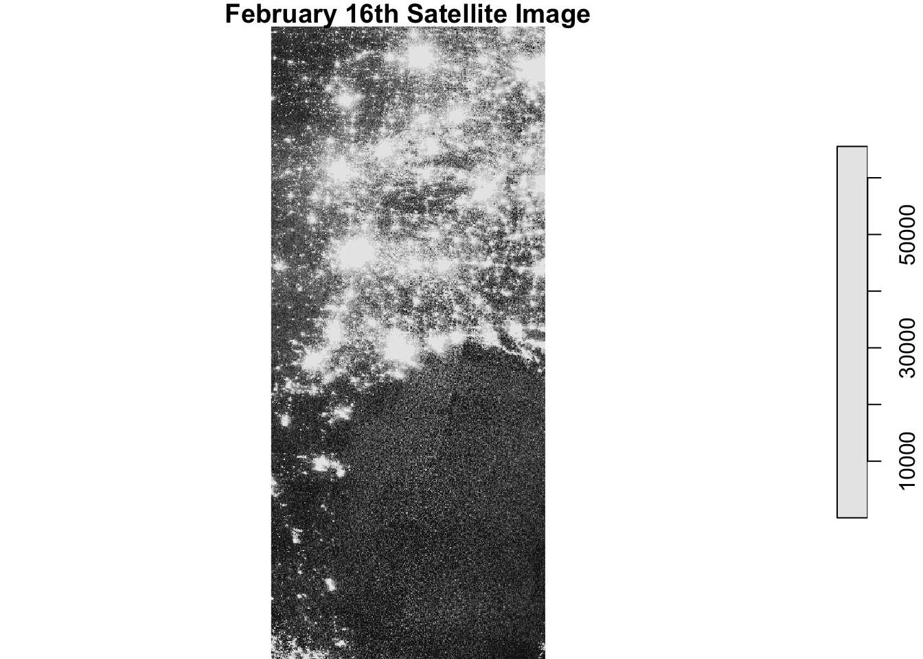
We used NASA’s Worldview to explore the data around the day of the storm. There were several days with too much cloud cover to be useful, but 2021-02-07 and 2021-02-16 provide two clear, contrasting images to visualize the extent of the power outage in Texas.

VIIRS data is distributed through NASA’s Level-1 and Atmospheric Archive & Distribution System Distributed Active Archive Center (LAADS DAAC). Many NASA Earth data products are distributed in 10x10 degree tiles in sinusoidal equal-area projection. Tiles are identified by their horizontal and vertical position in the grid. Houston lies on the border of tiles h08v05 and h08v06. We therefore needed to download two tiles per date.

Roads

Typically highways account for a large portion of the night lights observable from space (see Google’s Earth at Night). To minimize falsely identifying areas with reduced traffic as areas without power, we used a buffer to ignore areas near highways.

OpenStreetMap (OSM) is a collaborative project which creates publicly available geographic data of the world. Ingesting this data into a database where it can be subsetted and processed is a large undertaking. Fortunately, third party companies redistribute OSM data. We used Geofabrik’s download sites to retrieve a shapefile of all highways in Texas and prepared a Geopackage (.gpkg file) containing just the subset of roads that intersect the Houston metropolitan area.

Houses

We also obtained building data from OpenStreetMap. We again downloaded from Geofabrick and prepared a GeoPackage containing only houses in the Houston metropolitan area.

Socioeconomic

We cannot readily get socioeconomic information for every home, so instead we obtained data from the U.S. Census Bureau’s American Community Survey for census tracts in 2019. The folder ACS_2019_5YR_TRACT_48.gdb is an ArcGIS “file geodatabase”, a multi-file proprietary format that’s roughly analogous to a GeoPackage file. We used st_layers() to explore the contents of the geodatabase. Each layer contains a subset of the fields documents in the ACS metadata. The geodatabase contains a layer holding the geometry information, separate from the layers holding the ACS attributes. We had to combine the geometry with the attributes to get a feature layer that sf can use.

Assignment

Find locations of blackouts

We read the data in and converted it to a stars object, for compatibility with the sf package that we’ll use frequently in this analysis. We combined the tiles into a mosaic for each date (Feb 2, 2021, and Feb 16, 2021

Code

#reading in first tile from feb 7th
feb7_1 <-  data1 |> 
  st_as_stars()
#reading in second tile from feb 7th 
feb7_2 <- data2 |> 
  st_as_stars()

#combining tiles from feb 7th
feb7_mosaic <- st_mosaic(feb7_1, feb7_2)


#doing the same with first and second tiles from feb 16th
feb16_1 <- data3 |> 
  st_as_stars()

feb16_2 <- data4 |> 
  st_as_stars()


#combining them
feb16_mosaic <- st_mosaic(feb16_1, feb16_2)

#sanity check
plot(feb7_mosaic, main = "February 7th Satellite Image")

Code

plot(feb16_mosaic, main = "February 16th Satellite Image")

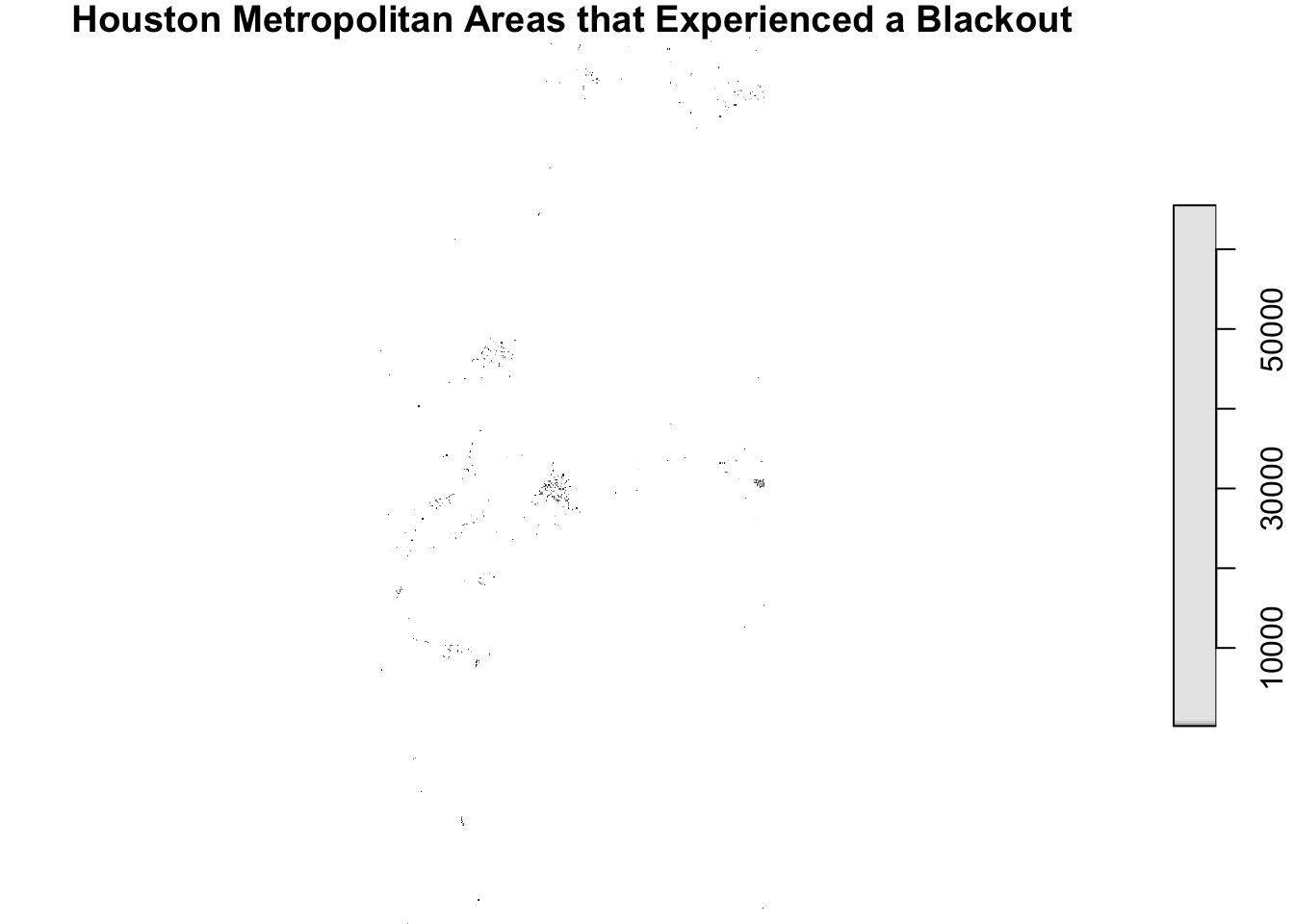
We then created a blackout mask to find the difference in the night light intensity between the two dates presumably caused by the storm. We then classified any location that experienced a drop of more than 200 nW cm^-2sr^-1 as a location that experienced a blackout. Any location that experienced less than 200 nW cm^-2sr^-1 was assigned NA

We then vectorized the blackout mask and fixed any invalid geometries

Code

#finding the change in night lights intensity - see what we get
difference_lights <- feb7_mosaic - feb16_mosaic
plot(difference_lights, main = "Difference in Light Intensity between February 7th and February 16th")

Code

#reclassify difference raster - assign NAs to all points experiencing a drop less than 200
difference_lights[difference_lights < 200] <-  NA
plot(difference_lights, main = "Houston Metropolitan Areas that Experienced a Blackout")

Code

#vectorize the blackout mask
blackout_mask <- st_as_sf(difference_lights) |> 
  st_make_valid()

We then cropped the vectorized map to our region of interest (Houston metropolitan area) using a bounding box, and assigned to it the same coordinate reference system as our night lights data. We then cropped the blackout mask to Houston, and reprojected the cropped dataset to EPSG:3083 (NAD83 / Texas Centric Albers Equal Area).

Code

#defining houston coordinates
houston <- cbind(x = c(-96.5, -96.5, -94.5, -94.5, -96.5), 
                         y = c(29, 30.5, 30.5, 29, 29))
#turning coordinates into polygon
houston <- st_sfc(st_polygon(list(houston)), crs = 4326)

#subsetting and masking houston
mask <- st_intersects(blackout_mask, houston, sparse = FALSE)
houston_subset <- blackout_mask[mask,]

#reprojecting
houston_reproj <- st_transform(houston_subset, crs = 3083)
plot(houston_reproj, main = "Blackouts in Houston")

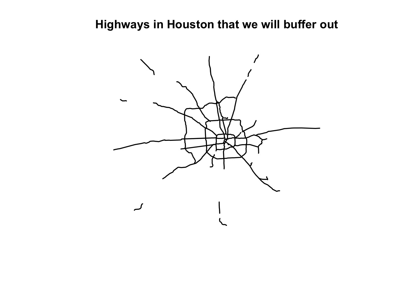
The next step was to exclude the highways from the blackout mask. We used an SQL query to load our highway data from the geopackage, and reprojected it to ESPG:3083. We then identified all areas within 200m of a highway using a buffer. After removing these areas, we were left with only the areas that experienced a blackout that are further than 200m from a highway.

Code

#reprojecting highways
highways_reproject <- st_transform(highways, crs = 3083)

#making undissolved buffers
highway_buffer <- st_union(st_buffer(highways_reproject, dist = 200))
plot(highway_buffer, main = "Highways in Houston that we will buffer out")

Code

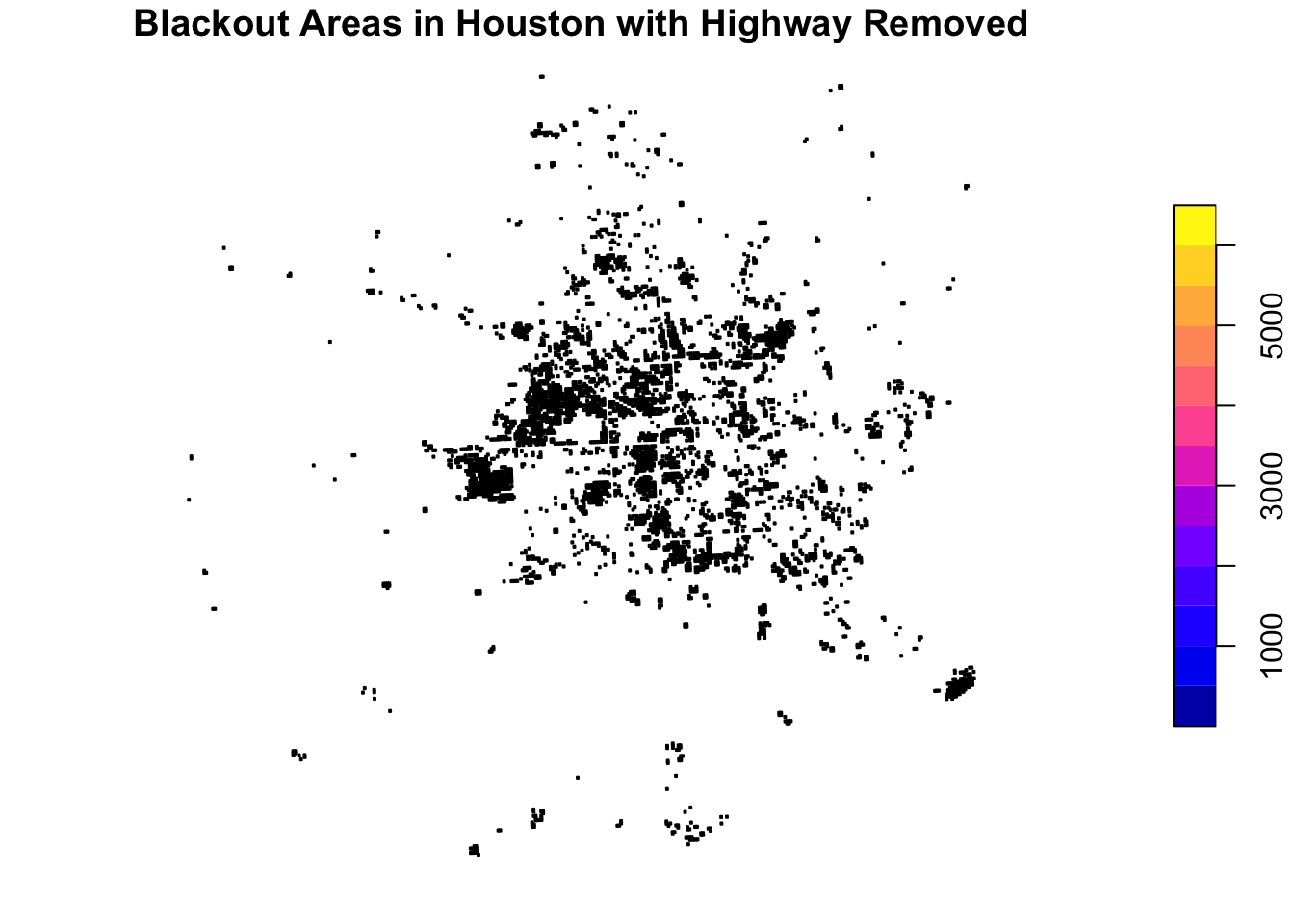
#plot area outside buffer
highway_blackouts <- houston_reproj[highway_buffer, op = st_disjoint]
plot(highway_blackouts, main = "Blackout Areas in Houston with Highway Removed")

To find the homes impacted by a blackout, we loaded the buildings dataset using another SQL query and only selected residential buildings. With the buildings dataset loaded and our blackout filter ready, we then filtered to homes within blackout areas. We were then able to count the number of impacted homes.

Code

#removing the buffered highways from the aoi
crop <- st_difference(houston_reproj, highway_buffer)

#subsetting here gives us all buildings>200m away from a highway that experienced a blackout
buildings_blackout <- buildings[crop, op = st_intersects]

#counting the number of residential buildings that got hit - 157970
print(paste0(nrow(buildings_blackout), ' buildings were affected by the blackouts'))

[1] "157970 buildings were affected by the blackouts"

Investigate socioeconomic factors

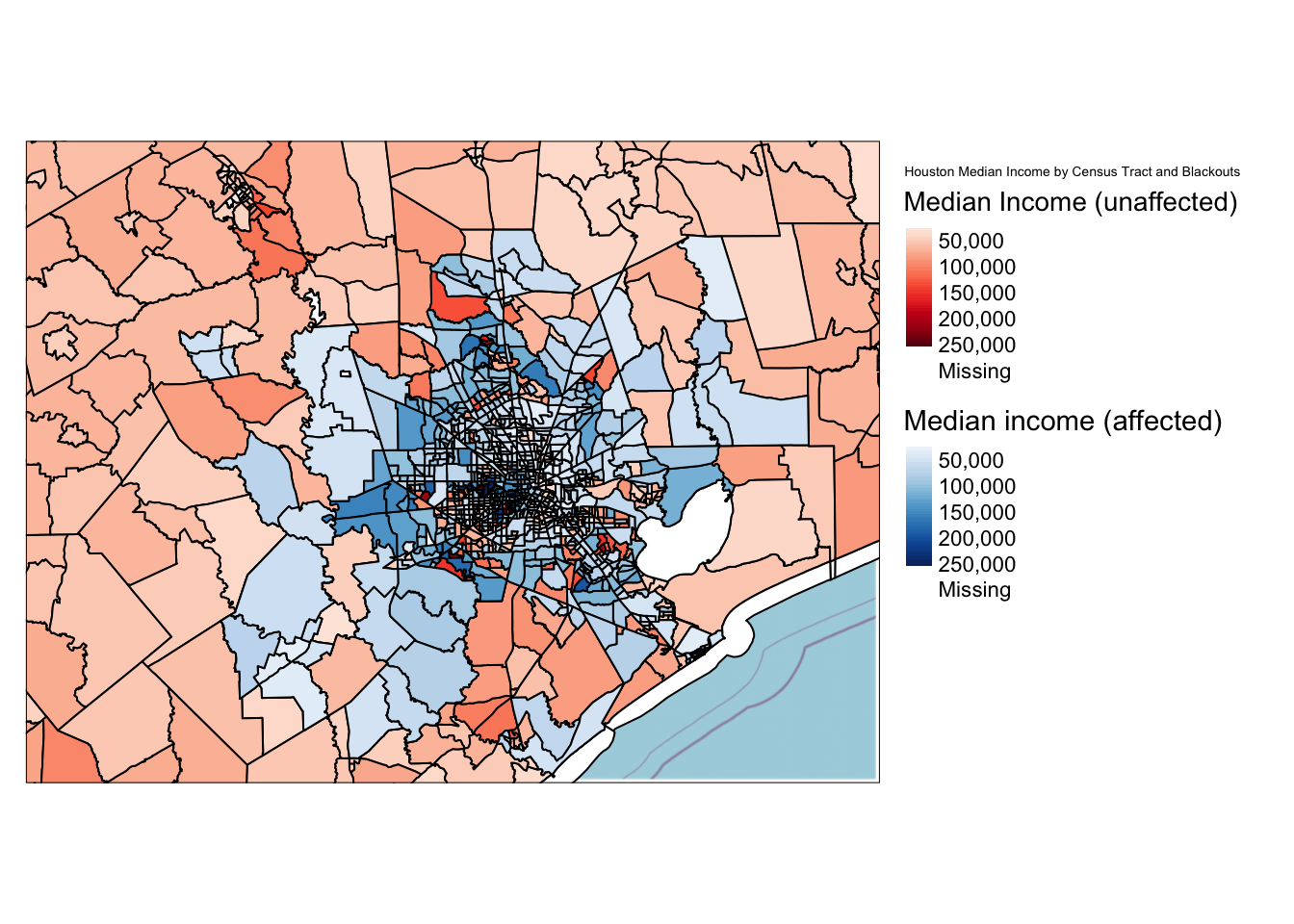
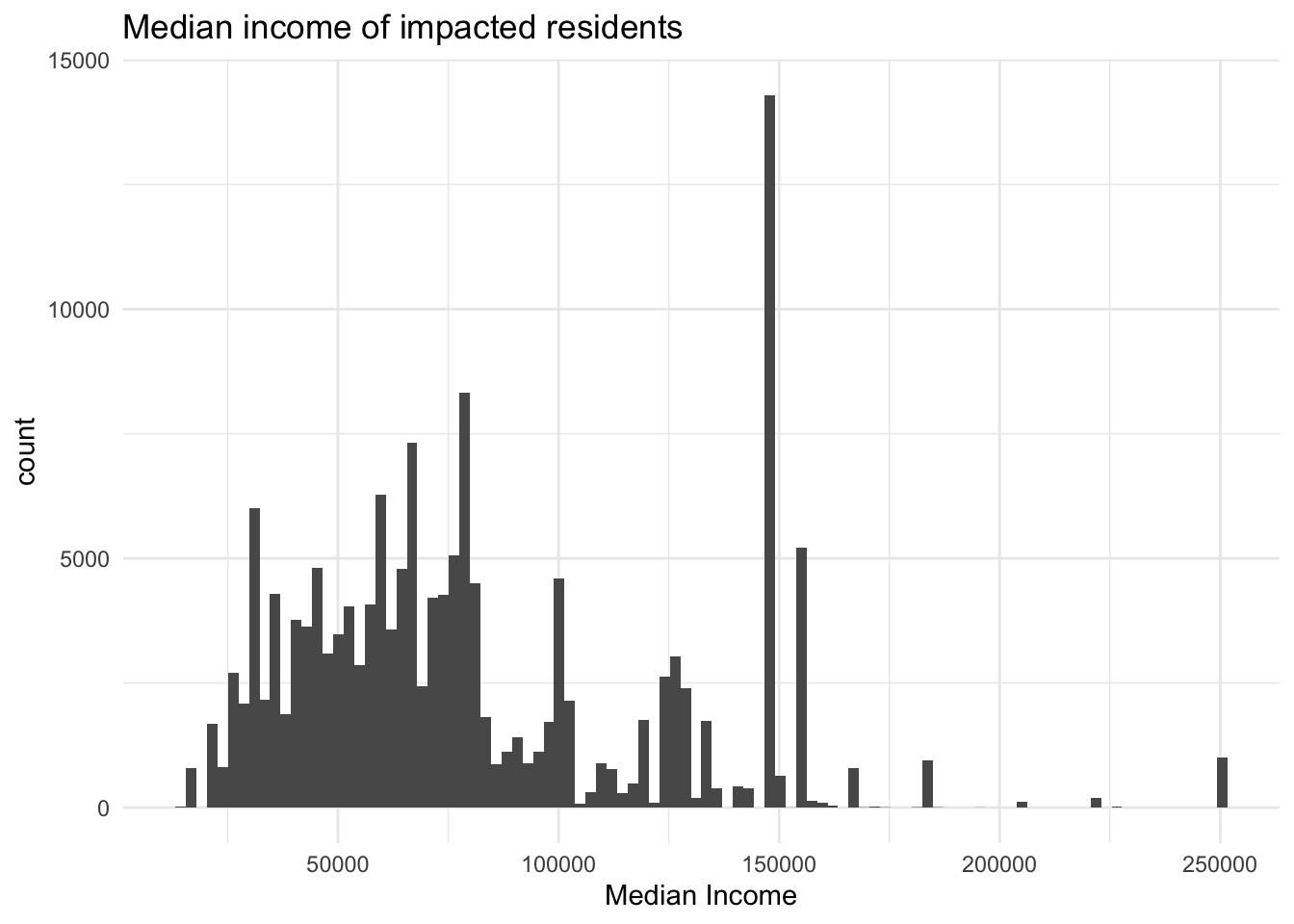
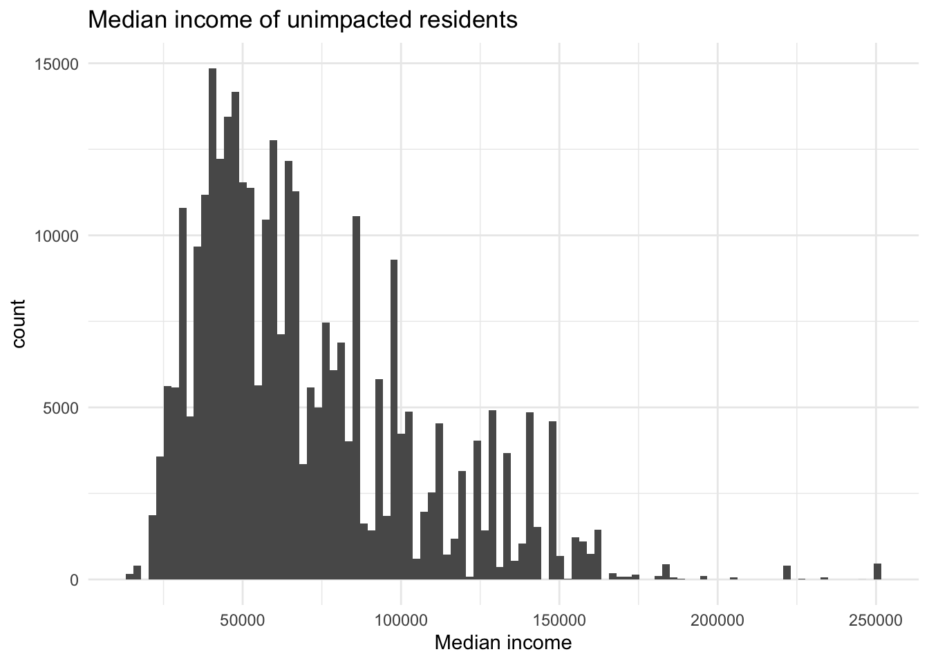
To investigate if blackouts caused by the storm were correlated with any socioeconomic factors, we first joined the income data to the census tract geometries, and find which of these tracts had blackouts. We then created a map of median income by census tract, designating which tracts had blackouts. We plotted the distribution of income in impacted and unimpacted tracts.

Code

#join
census_income <- left_join(census_geodata, geodata_income, by = c('GEOID_Data' = "GEOID")) 

#transform crs
census_income <- st_transform(census_income, crs = 3083)

# #Which tracts had blackouts?
data_blackouts <- st_join(buildings_blackout, census_income) |>
  mutate(blackout_present = if_else(is.na(osm_id), 0, 1))

#Buildings that didn't have any blackouts- manually used an anti-join
no_blackouts <- sapply(st_intersects(buildings, data_blackouts), function(x){length(x) == 0})
no_blackouts_2 <- buildings[no_blackouts,]

#plotting the buildings affected
blackout_buildings <- buildings_blackout[census_income,]

b2 <- census_income[buildings_blackout,]

#using our region we defined earlier + osm function to rasterize the bounding box
bounding_box <- st_bbox(houston) 
houston_map2 <- rosm::osm.raster(bounding_box)

#now for the map
tm_shape(houston_map2) + tm_rgb() + 
  tm_shape(census_income, bbox = bounding_box) +
  tm_polygons(col = 'income',
              colorNA = 'white',
              title = 'Median Income (unaffected)',
              palette= 'Reds', 
              style = 'cont') +
  tm_shape(b2, bbox = bounding_box) + 
  tm_style('col_blind') +
  tm_polygons(col = 'income',
              title = 'Median income (affected)',
              palette = 'Blues',
              style = 'cont') +
  tm_layout('Houston Median Income by Census Tract and Blackouts', legend.outside = TRUE)

Code

#distributions - impacted
impacted <- data_blackouts[buildings_blackout, op = st_intersects]
ggplot(data = impacted, aes(x = income)) + geom_histogram(bins = 100) + labs(title = 'Median income of impacted residents', x = 'Median Income', y = 'count') + theme_minimal()

Code

#income dist - unimpacted
unimpacted <- st_join(no_blackouts_2, census_income, join = st_intersects)
ggplot(data = unimpacted, aes(x = income)) + geom_histogram(bins = 100) + labs(title = 'Median income of unimpacted residents', x = 'Median income', y = 'count') + theme_minimal()

Over 150,000 buildings lost power in the Houston Metropolitan area due to the Texas 2021 February Winter storm. The distribution of median incomes between impacted and unimpacted residents appear to be similar. The median income of unaffected residents may be slightly higher on average than those who were affected by the blackouts. The limitations to this study include arbitrarily choosing a threshold in the change in light intensity between Feb 7 and Feb 16th, and basing our entire analyses off of data collected before the storm had finished hitting Houston. This limitation would systematically underestimate the extent of blackouts in Houston.

Footnotes

Wikipedia. 2021. “2021 Texas power crisis.” Last modified October 2, 2021. https://en.wikipedia.org/wiki/2021_Texas_power_crisis.↩︎